
I’ve been messing around with local LLMs on my 3090 for a while now — I have a growing collection of Qwen models on D:\LLM that I probably should be embarrassed about. A few weeks ago I stumbled across David Noel Ng’s LLM Neuroanatomy blog posts, where he showed that you can take a pretrained transformer and literally just re-run some of its middle layers a second time at inference, no retraining needed, and get meaningfully better outputs.
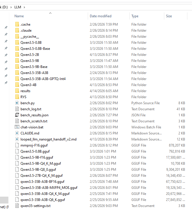
The D:\LLM folder. I should probably be embarrassed about this.
The idea is wild: the model’s weights don’t change. You just tell it “hey, run layers 15 through 21 again” and the hidden state gets another pass through those same weights. Ng showed this working on Qwen3.5-27B (a 64-layer model) with up to +15.6% improvement on combined math and emotional reasoning benchmarks.
Naturally, I wanted to know if this works on smaller models too. Welcome to Austin’s Nerdy Things, where we perform brain surgery on 4-billion-parameter language models to make them think twice.
Background: What Is RYS?
Ng’s technique is called RYS and the core concept is surprisingly simple. A normal transformer forward pass goes:
- Process input through layers 0, 1, 2, …, N-1 sequentially
- Done
With RYS, you pick a contiguous block in the middle — layers i through j-1 — and after the model finishes layer j-1, you jump back and re-execute layers i through N-1. Those middle layers run twice on the evolving hidden state.
The reason this can work is that transformer layers aren’t all doing the same thing. Ng’s work showed models have a recognizable three-phase anatomy:
- Early layers (~0-15% depth): Encoding. Converting tokens into contextualized representations. Repeating these produces garbage — the model tries to re-encode already-encoded stuff.
- Middle layers (~20-60% depth): Reasoning. The actual thinking. Repeating these is like giving the model extra time to work through the problem.
- Late layers (~70-100% depth): Decoding. Converting internal representations back into token predictions. Repeating these also produces garbage.
Ng found the sweet spot consistently in the middle, and his RYS repo provides all the tooling to test this — layer duplication wrappers, benchmark probe sets, the whole thing.
But his experiments were on a 27B model with 64 layers. I wanted to know: does this three-phase anatomy even exist at 4B scale? Can you exploit it on consumer hardware?
The Setup
Model: Qwen3-4B. I picked this one specifically because it’s a pure dense transformer (36 layers, 2560 hidden dim, GQA with 32 Q / 8 KV heads, RoPE, BF16). The Qwen3.5-2B has hybrid linear/full attention which would complicate things, and Qwen3-4B is in the same model family as Ng’s 27B target, which makes cross-scale comparison cleaner.
Hardware: My trusty RTX 3090 (24 GB VRAM). The model takes about 8.1 GB at baseline, which leaves plenty of room for the KV cache overhead from layer duplication.
Benchmarks: I used Ng’s probe sets from the RYS repo:
- Math-16: 16 hard math questions (square roots, cube roots, big multiplications) requiring single-integer answers. Scored with digit-level partial credit. No chain-of-thought allowed. Greedy decoding, 64 max new tokens.
- EQ-16: 16 EQ-Bench scenarios — complex social dialogues where the model predicts 4 emotion intensities on a 0-10 scale. Max 256 new tokens.
I used /no_think to disable Qwen3’s thinking mode so we’re measuring raw single-pass capability, and greedy decoding (do_sample=False), which I verified is perfectly deterministic across 5 runs on the same input. No need for multi-run variance testing.
The sweep: All 667 valid (i, j) configurations for a 36-layer model, including baseline (0, 0). Every config runs all 32 probe questions. I added early stopping that triggers if the first 2 math probes both produce garbage (saves about 30% of wall time on broken configs). The scanner saves results to JSON after every single config — resume-friendly for when Windows decides it’s update time.
Total sweep time: about 9 hours on a single 3090. Claude helped me write the scanner script (with me providing the architecture decisions and Ng’s RYS library doing the heavy lifting on layer manipulation).
Baseline Scores
Before messing with anything, Qwen3-4B scores:
| Probe | Score |
|---|---|
| Math-16 | 0.305 |
| EQ-16 | 0.749 |
| Combined | 1.054 |
The math score looks low, but these are genuinely hard problems (like “what is the cube root of 1019330085047 times 31?”) and the scorer gives partial credit for getting digits right. The EQ score is actually solid — Qwen3-4B is pretty decent at predicting emotional dynamics even without chain-of-thought.
The Heatmaps
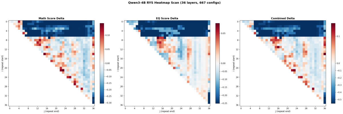
Here’s where it gets fun. I swept all 667 configs and plotted the results as heatmaps. Each cell is one (i, j) configuration. Red means improvement over baseline. Blue means degradation. The x-axis is j (where the repeated block ends) and the y-axis is i (where it starts).

Left: math delta. Center: EQ delta. Right: combined delta. Red = improvement, blue = degradation. 667 configs, 36 layers.
Three things jumped out immediately.
1. The three-phase anatomy is clearly present at 4B scale
The top-left corner (early layers duplicated with wide spans) is deep blue — that’s the encoding zone. The bottom-right corner (late layers) is also blue — that’s the decoding zone. The productive region runs diagonally through the middle. This is exactly the encode / reason / decode structure Ng found at 27B.
Layers 0-6 are the encoding wall. Repeat anything starting before layer 5 with a wide span and the model outputs garbage. Layers 30+ are decoding territory — also garbage if you repeat there. The productive zone lives between layers ~5 and ~27, spanning roughly 60% of the model.
2. Math and EQ have different hot zones
This was something I wasn’t expecting. The math heatmap shows gains across a broad band from mid-stack to upper layers. The EQ heatmap’s gains concentrate in a tighter region around layers 7-16. The combined heatmap shows three distinct hot zones:
- Zone A (layers 7-15, ~19-42% depth): Strong EQ gains, moderate math
- Zone B (layers 15-20, ~42-56% depth): Balanced improvement on both
- Zone C (layers 21-27, ~58-75% depth): Strong math gains, EQ roughly neutral
So the model’s “emotional processing” lives slightly earlier in the stack than its “mathematical processing.” That’s a cool finding — different kinds of reasoning occupy different layer ranges even in a small model.
3. The encoding wall is a cliff, not a slope
The transition from “productive duplication” to “catastrophic failure” happens over 1-2 layers. Layer 5 duplication helps. Layer 3 duplication tanks the model. There’s basically no gradient — it’s a cliff edge. Ng observed something similar at 27B but it’s even more pronounced at 4B scale.
The Pareto Frontier
Not all improvements are worth the extra latency. Each extra layer traversal costs time. The practical question is: how much bang per buck?
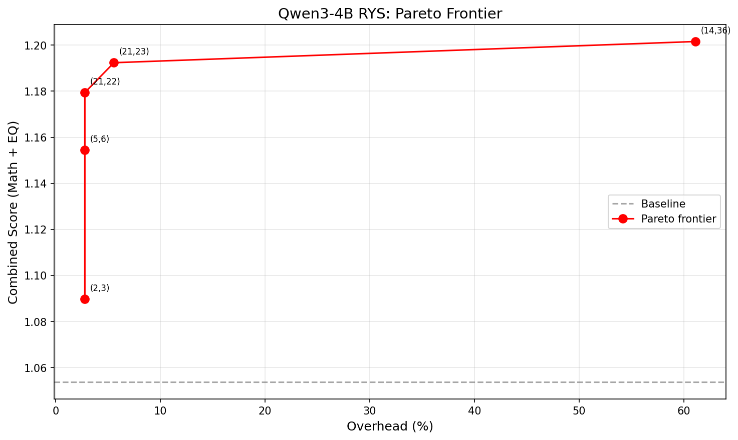
X-axis: overhead (%). Y-axis: combined score. The curve is sharply concave — almost all the benefit comes from the first 1-2 extra layers.
| Size | Config (i,j) | Extra layers | Overhead | Combined | Improvement |
|---|---|---|---|---|---|
| XS | (2,3) | 1 | 2.8% | 1.090 | +3.4% |
| S | (5,6) | 1 | 2.8% | 1.154 | +9.6% |
| M | (21,22) | 1 | 2.8% | 1.179 | +11.9% |
| L | (21,23) | 2 | 5.6% | 1.192 | +13.2% |
| XL | (14,36) | 22 | 61.1% | 1.202 | +14.0% |
The winner is (21,22): just repeat layer 21 once. That’s +11.9% combined improvement at 2.8% latency overhead. One single extra layer forward pass. That’s it.
Going from 1 extra layer to 2 buys another 1.3 percentage points. Going from 2 extra layers to 22 — literally 10x the overhead — buys only 0.8 more. The returns collapse fast. Look at that Pareto chart — the curve is basically flat after the first couple of points.
Single-Layer Repeats: The 4B Surprise
This is where things get really interesting, and where the results diverge most from Ng’s 27B findings.
Ng reported that single-layer repeats at 27B “almost never help.” You need to duplicate a contiguous block of at least 2-3 layers to see meaningful improvement at that scale.
At 4B? 14 out of 35 single-layer repeats beat baseline. Here are the top performers:
| Layer | Config | Combined delta |
|---|---|---|
| 21 | (21,22) | +0.126 |
| 5 | (5,6) | +0.101 |
| 24 | (24,25) | +0.100 |
| 26 | (26,27) | +0.073 |
| 19 | (19,20) | +0.071 |
| 22 | (22,23) | +0.063 |
| 20 | (20,21) | +0.057 |
| 17 | (17,18) | +0.049 |
Layers 5 and 17-26 — nearly the entire mid-to-late stack — all produce meaningful gains when repeated individually. That’s a wide, diffuse productive zone spanning about 60% of the model.
My interpretation: smaller models have less specialized layers. At 27B with 64 layers, each layer does something specific enough that repeating just one doesn’t help much — you need a coherent block. At 4B with 36 layers, individual layers carry more general-purpose reasoning capacity. A single extra pass through one of them is already enough to bump quality.
This is arguably the most practically useful finding from the whole experiment. For small models, even the simplest possible intervention works.
How This Compares to Ng’s 27B Results
| Property | Qwen3-4B (36 layers) | Qwen3.5-27B (64 layers) |
|---|---|---|
| Three-phase anatomy | Yes, clearly visible | Yes |
| Encoding wall | Layers 0-6 (~0-17%) | ~first 15% |
| Best single-layer | (21,22) = +11.9% | Rarely productive |
| Best absolute | (14,36) = +14.0% at 61% overhead | ~+15.6% at ~15.6% overhead |
| Best efficiency | (21,22) = +11.9% at 2.8% overhead | Layer 33 = +1.5% |
| Productive single layers | 14/35 (40%) | Rare |
| Efficiency curve shape | Sharply concave | Roughly linear to ~10 layers |
The biggest difference is the shape of the efficiency curve. At 27B, adding more repeated layers gives roughly linear improvement up to about 10 extra layers — there’s a real reason to invest in multi-layer duplication. At 4B, the curve is sharply concave. Almost all the benefit comes from the very first extra layer. After that, you’re paying a lot of overhead for very little gain.
This makes intuitive sense. A bigger model has more specialized layers where repetition compounds — each one contributes something distinct. A smaller model gets most of its benefit from a single extra pass through its most general-purpose reasoning layer, and additional passes hit diminishing returns because those layers are doing similar work.
What This Means If You Want to Use It
If you’re deploying a small dense model and want better reasoning at minimal cost:
- Find the model’s “layer 21.” Run a quick single-layer sweep on your target model. It takes minutes per config.
- Repeat that one layer. At 2.8% latency overhead, this is basically free.
- Don’t over-invest in multi-layer duplication at small scale. The second extra layer buys way less than the first.
For framework implementers: this is a ~10-line change to a model’s forward pass. No weight changes, no retraining, no meaningful VRAM increase. It should be a first-class inference option in llama.cpp, vLLM, ExLlama, etc.
Caveats
I want to be upfront about what this doesn’t prove:
- One model, one family. These results are Qwen3-4B specific. The three-phase anatomy probably generalizes (Ng showed it on multiple architectures), but the exact layer numbers won’t. Every model needs its own sweep.
- Small probe sets. 16 math + 16 EQ questions. Enough for relative ordering of configs, but the absolute scores have meaningful variance. Validate on larger benchmarks before deploying.
- Greedy decoding only. Sampling might interact differently with layer duplication. I haven’t tested that.
- BF16 only. Quantized models might behave differently — layer duplication could amplify quantization errors.
- No multi-block compositions. Ng’s beam search finds configs that repeat two different blocks (e.g., layers 30-34 AND 43-45). I only tested single contiguous blocks. The multi-block space at 4B is unexplored.
- RoPE positions aren’t adjusted. The model sees the same position IDs on the repeated pass. This works empirically but the theoretical interaction is unclear.
Reproducing This
Everything runs on a single 3090 (or any 24GB+ GPU):
- Model: Qwen/Qwen3-4B in BF16 (~8 GB VRAM)
- Tooling: Ng’s RYS repo for the layer duplicator and probe datasets
- Scanner: Custom
rys_scan.py— single file, ~460 lines, resume-friendly - Analysis: Custom
rys_analyze.py— heatmaps, Pareto frontier, markdown summary - Dependencies: PyTorch, transformers, matplotlib, numpy
- Wall time: ~9 hours for the full 667-config sweep
The scanner loads the model once, pre-tokenizes all probes, then iterates through configs. Each config wraps the base model with a layer-index remapping (no weight copies, just pointer rearrangement), runs all probes greedy, scores, and saves. Resume works by checking which config keys already exist in the results JSON.
What’s Next
A few obvious follow-ups I’m thinking about:
- Multi-block beam search at 4B. Does combining layers 5-6 and 21-22 compound the gains?
- Cross-scale comparison. Run the same sweep on Qwen3.5-2B (hybrid attention), Qwen3.5-9B, maybe a non-Qwen model. See how the efficiency curve changes with scale.
- Train-time loop exposure. Train a small model where specific layers are looped during training, compare with inference-time-only duplication.
- Integration with inference frameworks. llama.cpp, vLLM, and ExLlama already manage layer weights — adding a “repeat layer N” flag should be pretty straightforward.
The broader takeaway is that transformer layers aren’t interchangeable. They have structure, and that structure is legible even at small scale. You can exploit it at inference time with zero retraining, and the cost is basically nothing.
Layer 21 thinks twice. The model gets smarter. That’s the whole trick.
This work builds directly on David Noel Ng’s RYS and LLM Neuroanatomy series — go read those if you haven’t, they’re excellent. Related academic work: Reasoning with Latent Thoughts and LoopFormer. Data, scanner script, and full results available on GitHub.