Categories
AI homelab Programming Python

Building DIMMsum: a price tracker for used server RAM on eBay

This project exists because I bought 30 sticks of 16GB DDR4-3200 RDIMM for an EPYC build in early April: an r/homelabsales find at $80 a stick, which was a fair price that day. The problem is that “that day” turned out to be the exact top of the market. Buying the top is pretty standard for me. Then the server wouldn’t POST with at least 4 of the sticks installed, and of the 16 that made it in, 4 more start throwing ECC errors the moment I do anything memory-heavy (LLM inferencing, which is of course why I bought them). There are still 6 untested sticks in the box. I knew the going rate; what I couldn’t see was where prices were headed or which sticks would actually work. A price tracker with real sold history fixes at least the first problem.

Beyond my own bad luck, the general problem is that eBay search results for server RAM are a mess. “32GB (2x16GB)” is two 16GB sticks, not one 32GB stick. The same 2666 MT/s speed shows up as DDR4-2666, PC4-21300, PC4-2666V, or just “2666V” depending on the seller’s mood. Lots of 8, lots of 32, single sticks, and “FOR PARTS” boards are all mixed together in the same results. Comparing actual price per gigabyte across all of that by hand is miserable.

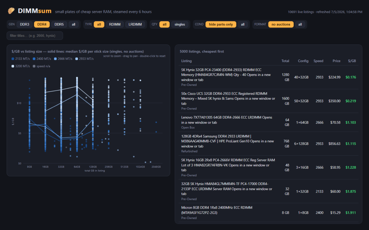
LabGopher solved this years ago for whole servers, and I have wanted the RAM equivalent basically forever. So I built it: DIMMsum, a free site that scrapes eBay every 6 hours, normalizes the listing titles with an LLM, and charts everything as $/GB with median market lines per speed grade.

Welcome to Austin’s Nerdy Things, where we deploy a browser farm and a language model to avoid doing mental math on eBay listings.
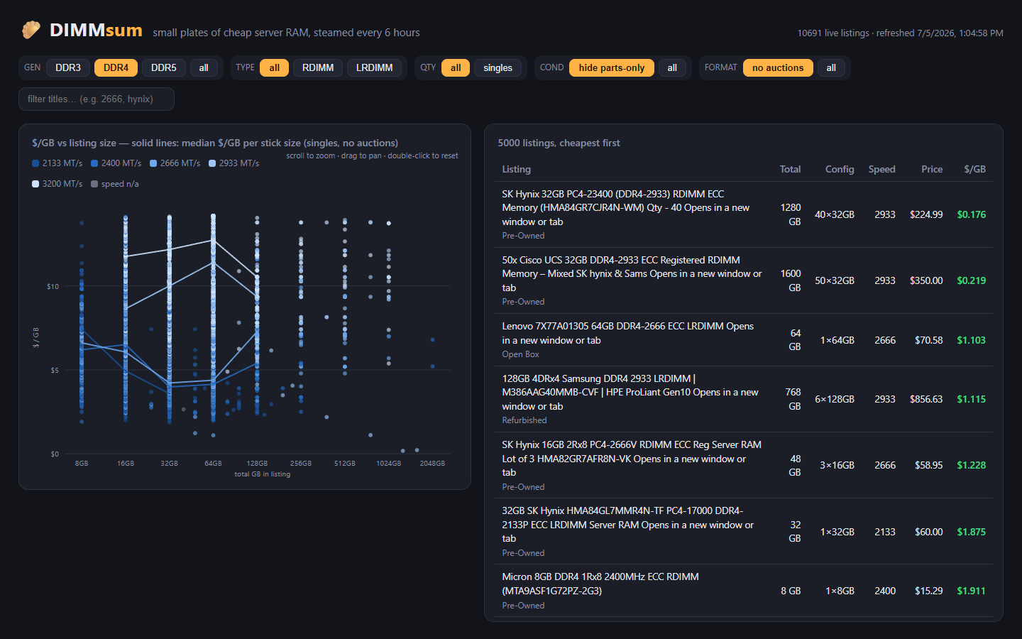
DIMMsum homepage: $/GB scatter of live eBay listings colored by speed, with median market lines and the cheapest-first table

My first attempt (2024) was bad

This is actually my second run at scraping eBay. Back in 2024 I wrote a requests + BeautifulSoup scraper that pulled search results through free SOCKS proxies from public proxy lists. It mostly worked, in the sense that it is technically still running on an LXC in my basement, appending to a parse.log that is now 636MB. The proxies were garbage (free proxies are free for a reason), the regex title parsing was wrong constantly, and I never did anything with the data. Classic.

Two things changed since then: eBay got much more aggressive about blocking scrapers, and LLMs got cheap enough to throw at every single listing title. Both of those turned out to matter a lot.

eBay does not want to be scraped (by robots that look like robots)

The 2024 approach is completely dead in 2026. Plain HTTP clients like requests do not even get to say hello anymore – eBay identifies them as robots essentially instantly and serves a 403 or the “Pardon Our Interruption” page. My first attempts with an automated browser got generic eBay error pages on search URLs too, while the exact same URLs worked fine by hand. That one had me confused for a while.

I am going to spare you the play-by-play here, partly because it would be a bot-evasion cookbook published by a site that participates in eBay’s own affiliate program, which seems unwise. The short version: the fix was embarrassingly simple, and it amounted to using a real browser (Playwright driving full Chromium) and having it behave like a polite human instead of a robot in a hurry. Take the path a person would take, slow down, keep the footprint small. No proxies, no stealth plugins, one IP, 3-6 second randomized delays between pages, and eBay has been perfectly happy serving me 240 listings per page ever since – a few hundred page loads a day, total.

The query matrix (or: making the search do half the parsing)

Instead of one broad “ddr4 rdimm” search, DIMMsum runs 51 very specific queries, one per capacity + speed + module type combo:

32gb (2666,pc4-21300,2666v) rdimm -2x16 -4x8 -8x4

The parenthesized part is eBay OR syntax covering the speed synonyms, and the negative terms exclude kit notation so results skew toward true single sticks. The neat part is that each query doubles as a weak label: if a listing was found by the 32GB 2666 RDIMM query but parses out as a 16GB stick, something is off (a lot, a mislabel, or a parse bug), and it gets flagged with a little warning icon in the UI instead of silently polluting the chart.

LLM title parsing for $0.09 per thousand listings

Here is a real title from the database:

2048GB 128x16GB DDR3 PC3L-10600R ECC Reg Server Memory RAM

That is 128 sticks of 16GB low-voltage DDR3-1333 RDIMM. My 2024 regex parser had no chance. The domain rules are genuinely fiddly: a PC3L prefix means low voltage, but a trailing L on the PC number (PC3-14900L) means LRDIMM, and both can appear in the same token. Kit notation states the total first. “LOT” without a count does not mean quantity greater than one. Part numbers are more authoritative than the title text around them.

Rather than encoding all that in regex, every title goes through DeepSeek (deepseek-v4-flash, their cheap model) with a system prompt full of those domain rules, returning structured JSON validated by a pydantic schema:

class RamSpec(BaseModel):
    is_ram: bool          # False for trays, heat spreaders, "for parts" boards
    qty: Optional[int]    # lot/kit aware stick count
    per_stick_gb: Optional[int]
    total_gb: Optional[int]
    ddr_gen: Optional[int]        # 3, 4, 5
    module_type: Optional[str]    # RDIMM | LRDIMM | UDIMM | SODIMM
    speed_mts: Optional[int]      # PC4-21300 -> 2666
    # ... rank, voltage, ECC, part number

Titles are batched 25 per API call with an index round-trip check so a misaligned response fails loudly instead of assigning specs to the wrong listings. Against a hand-labeled fixture set it scored 97.4% field accuracy on the first eval run, and the misses were fields that only existed encoded inside part numbers (a future deterministic PN-decode layer will catch those).

The economics are the part that still makes me smile. At roughly $0.09 per 1,000 titles, the total LLM bill for parsing every listing DIMMsum has ever seen is about two dollars. This pipeline was not possible on a hobby budget three years ago; now it is basically free.

The plumbing

Everything lands in Postgres on my Proxmox cluster (one VM for the scraper + web app, one for the database). A systemd timer scrapes every 6 hours, and each run records a price snapshot per listing, which means DIMMsum builds its own price history for every item it tracks. The web side is FastAPI plus one vanilla JavaScript file. No framework. The whole site is a scatter chart, a table, and some server-rendered spec pages.

Current state of the database after a few days of running:

MetricCount
RAM listings tracked10,697
Price snapshots104,475
Search queries per run51
Scrape frequencyevery 6 hours
LLM parse cost, lifetime~$2

Claude (Fable 5, via Claude Code) wrote most of this code with me over a few evenings. The architecture arguments were real arguments and it lost some of them, but I will happily credit it with the claim-column work queue pattern that lets me run parallel parse workers against Postgres without them stepping on each other.
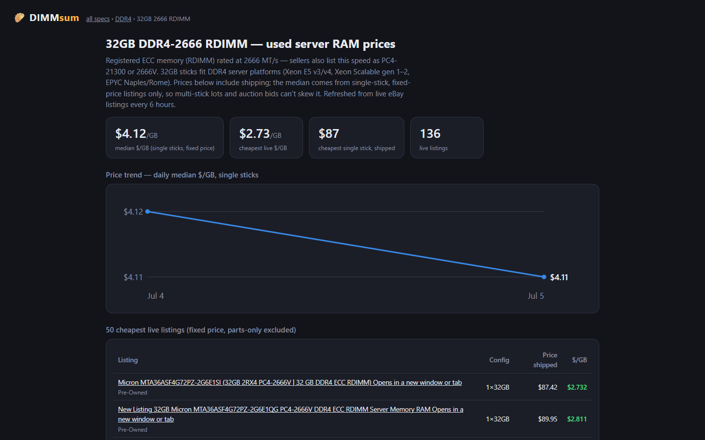
The spec page for 32GB DDR4-2666 RDIMM: median and cheapest stat tiles, daily price trend, and the 50 cheapest live listings

Sold prices (the part I am most excited about)

Active listing prices tell you what sellers are asking. Sold prices tell you what buyers actually paid, and those are very different numbers on eBay.

I assumed for months that scraping sold/completed listings was off the table and never actually tested it. Turns out the same polite-human browsing approach handles the sold/completed view just fine, and eBay hands you sold prices with dates, 240 per page. I was wrong for months for no reason. Test your assumptions, folks.

So as of this week DIMMsum also harvests sold listings weekly into their own table. The first sweep pulled in over 8,000 real sales, and the sold history goes back further than the ~90 days I expected (most of the usable volume reaches back to late 2025). That data is going to power a monthly “state of the used RAM market” report: median $/GB by SKU, month over month, from real transactions. The June data already shows 8GB DDR4-2133 RDIMMs sliding from $3.50/GB in April to $3.12 in June, and that is exactly the kind of thing I want a monthly email about.

There is a signup box at the bottom of dimmsum.com for exactly that report. One email a month, actual data, no other nonsense.

Disclosure and what’s next

The site is monetized with eBay Partner Network affiliate links: if you click through and buy, eBay pays a commission. That is the entire business model. Free site, no ads, no accounts, and the full disclosure lives in the footer.

Next up: the monthly sold-price report, a storage version (same idea, $/TB for used enterprise SSDs and HDDs, already in progress as a separate project), and a part-number decode table to squeeze out the last few percent of parse accuracy.

Go find some cheap RDIMMs at dimmsum.com. My benchmark SKU (32GB DDR4-2666 RDIMM singles) has a median around $132 a stick right now with the floor meaningfully below that, and now I get to watch the market instead of refreshing eBay searches like an animal.
Categories
AI Python

One Layer, +12%: What 667 Configs Reveal About Small LLM Anatomy

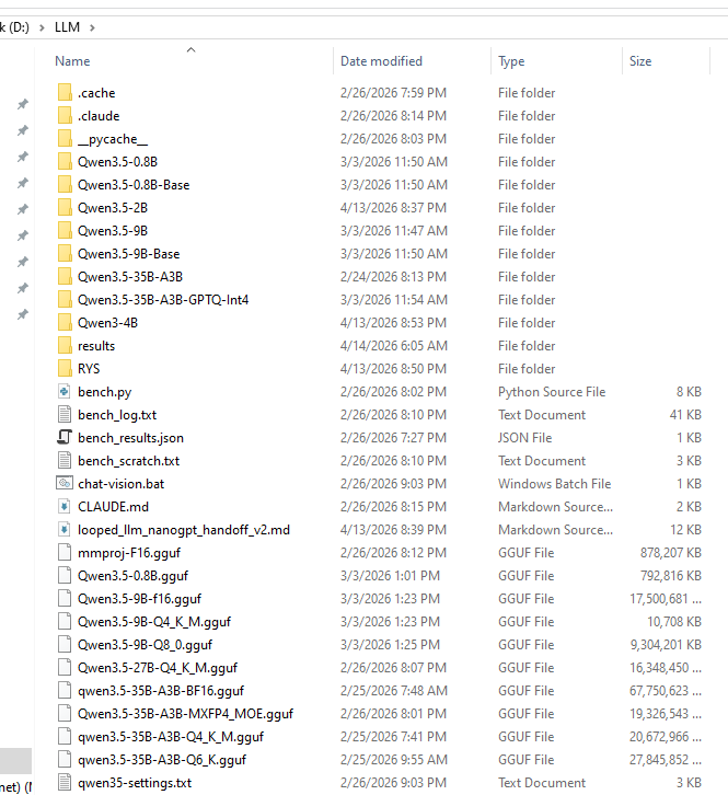
I’ve been messing around with local LLMs on my 3090 for a while now — I have a growing collection of Qwen models on D:\LLM that I probably should be embarrassed about. A few weeks ago I stumbled across David Noel Ng’s LLM Neuroanatomy blog posts, where he showed that you can take a pretrained transformer and literally just re-run some of its middle layers a second time at inference, no retraining needed, and get meaningfully better outputs.

Windows Explorer showing my D:\LLM folder stuffed with Qwen models and GGUF files

The D:\LLM folder. I should probably be embarrassed about this.

The idea is wild: the model’s weights don’t change. You just tell it “hey, run layers 15 through 21 again” and the hidden state gets another pass through those same weights. Ng showed this working on Qwen3.5-27B (a 64-layer model) with up to +15.6% improvement on combined math and emotional reasoning benchmarks.

Naturally, I wanted to know if this works on smaller models too. Welcome to Austin’s Nerdy Things, where we perform brain surgery on 4-billion-parameter language models to make them think twice.


Background: What Is RYS?

Ng’s technique is called RYS and the core concept is surprisingly simple. A normal transformer forward pass goes:

  1. Process input through layers 0, 1, 2, …, N-1 sequentially
  2. Done

With RYS, you pick a contiguous block in the middle — layers i through j-1 — and after the model finishes layer j-1, you jump back and re-execute layers i through N-1. Those middle layers run twice on the evolving hidden state.

The reason this can work is that transformer layers aren’t all doing the same thing. Ng’s work showed models have a recognizable three-phase anatomy:

  • Early layers (~0-15% depth): Encoding. Converting tokens into contextualized representations. Repeating these produces garbage — the model tries to re-encode already-encoded stuff.
  • Middle layers (~20-60% depth): Reasoning. The actual thinking. Repeating these is like giving the model extra time to work through the problem.
  • Late layers (~70-100% depth): Decoding. Converting internal representations back into token predictions. Repeating these also produces garbage.

Ng found the sweet spot consistently in the middle, and his RYS repo provides all the tooling to test this — layer duplication wrappers, benchmark probe sets, the whole thing.

But his experiments were on a 27B model with 64 layers. I wanted to know: does this three-phase anatomy even exist at 4B scale? Can you exploit it on consumer hardware?


The Setup

Model: Qwen3-4B. I picked this one specifically because it’s a pure dense transformer (36 layers, 2560 hidden dim, GQA with 32 Q / 8 KV heads, RoPE, BF16). The Qwen3.5-2B has hybrid linear/full attention which would complicate things, and Qwen3-4B is in the same model family as Ng’s 27B target, which makes cross-scale comparison cleaner.

Hardware: My trusty RTX 3090 (24 GB VRAM). The model takes about 8.1 GB at baseline, which leaves plenty of room for the KV cache overhead from layer duplication.

Benchmarks: I used Ng’s probe sets from the RYS repo:

  • Math-16: 16 hard math questions (square roots, cube roots, big multiplications) requiring single-integer answers. Scored with digit-level partial credit. No chain-of-thought allowed. Greedy decoding, 64 max new tokens.
  • EQ-16: 16 EQ-Bench scenarios — complex social dialogues where the model predicts 4 emotion intensities on a 0-10 scale. Max 256 new tokens.

I used /no_think to disable Qwen3’s thinking mode so we’re measuring raw single-pass capability, and greedy decoding (do_sample=False), which I verified is perfectly deterministic across 5 runs on the same input. No need for multi-run variance testing.

The sweep: All 667 valid (i, j) configurations for a 36-layer model, including baseline (0, 0). Every config runs all 32 probe questions. I added early stopping that triggers if the first 2 math probes both produce garbage (saves about 30% of wall time on broken configs). The scanner saves results to JSON after every single config — resume-friendly for when Windows decides it’s update time.

Total sweep time: about 9 hours on a single 3090. Claude helped me write the scanner script (with me providing the architecture decisions and Ng’s RYS library doing the heavy lifting on layer manipulation).


Baseline Scores

Before messing with anything, Qwen3-4B scores:

ProbeScore
Math-160.305
EQ-160.749
Combined1.054

The math score looks low, but these are genuinely hard problems (like “what is the cube root of 1019330085047 times 31?”) and the scorer gives partial credit for getting digits right. The EQ score is actually solid — Qwen3-4B is pretty decent at predicting emotional dynamics even without chain-of-thought.


The Heatmaps

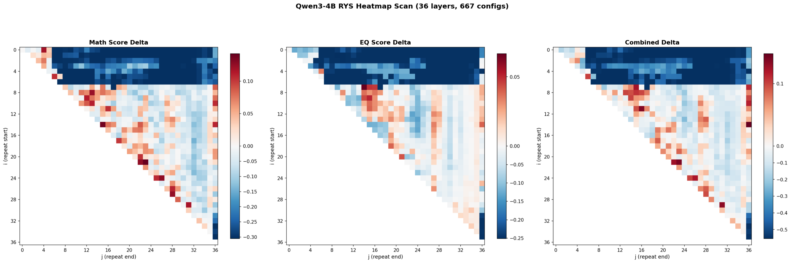
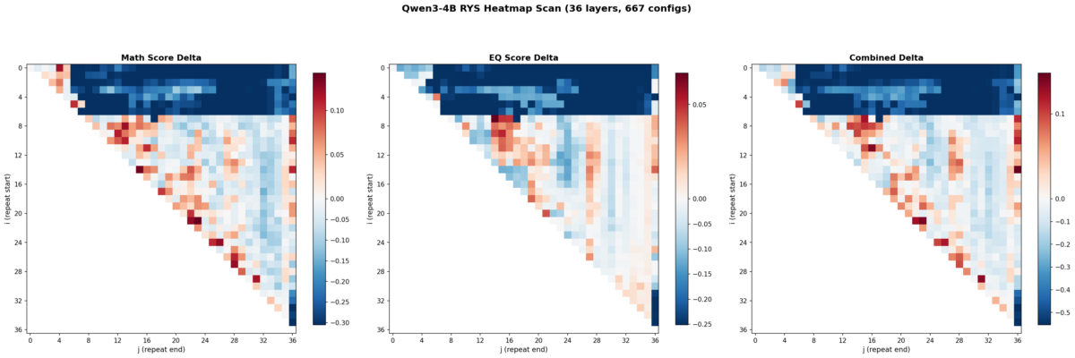
Here’s where it gets fun. I swept all 667 configs and plotted the results as heatmaps. Each cell is one (i, j) configuration. Red means improvement over baseline. Blue means degradation. The x-axis is j (where the repeated block ends) and the y-axis is i (where it starts).

Qwen3-4B RYS heatmap triptych -- math, EQ, and combined score deltas vs baseline across 667 configurations

Left: math delta. Center: EQ delta. Right: combined delta. Red = improvement, blue = degradation. 667 configs, 36 layers.

Three things jumped out immediately.

1. The three-phase anatomy is clearly present at 4B scale

The top-left corner (early layers duplicated with wide spans) is deep blue — that’s the encoding zone. The bottom-right corner (late layers) is also blue — that’s the decoding zone. The productive region runs diagonally through the middle. This is exactly the encode / reason / decode structure Ng found at 27B.

Layers 0-6 are the encoding wall. Repeat anything starting before layer 5 with a wide span and the model outputs garbage. Layers 30+ are decoding territory — also garbage if you repeat there. The productive zone lives between layers ~5 and ~27, spanning roughly 60% of the model.

2. Math and EQ have different hot zones

This was something I wasn’t expecting. The math heatmap shows gains across a broad band from mid-stack to upper layers. The EQ heatmap’s gains concentrate in a tighter region around layers 7-16. The combined heatmap shows three distinct hot zones:

  • Zone A (layers 7-15, ~19-42% depth): Strong EQ gains, moderate math
  • Zone B (layers 15-20, ~42-56% depth): Balanced improvement on both
  • Zone C (layers 21-27, ~58-75% depth): Strong math gains, EQ roughly neutral

So the model’s “emotional processing” lives slightly earlier in the stack than its “mathematical processing.” That’s a cool finding — different kinds of reasoning occupy different layer ranges even in a small model.

3. The encoding wall is a cliff, not a slope

The transition from “productive duplication” to “catastrophic failure” happens over 1-2 layers. Layer 5 duplication helps. Layer 3 duplication tanks the model. There’s basically no gradient — it’s a cliff edge. Ng observed something similar at 27B but it’s even more pronounced at 4B scale.


The Pareto Frontier

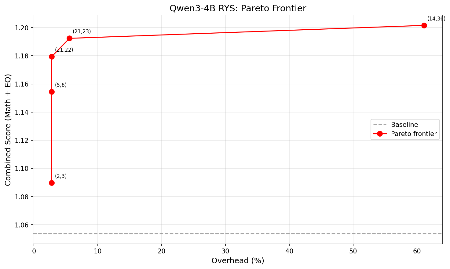
Not all improvements are worth the extra latency. Each extra layer traversal costs time. The practical question is: how much bang per buck?

Qwen3-4B RYS Pareto frontier -- overhead percentage vs combined score

X-axis: overhead (%). Y-axis: combined score. The curve is sharply concave — almost all the benefit comes from the first 1-2 extra layers.

SizeConfig (i,j)Extra layersOverheadCombinedImprovement
XS(2,3)12.8%1.090+3.4%
S(5,6)12.8%1.154+9.6%
M(21,22)12.8%1.179+11.9%
L(21,23)25.6%1.192+13.2%
XL(14,36)2261.1%1.202+14.0%

The winner is (21,22): just repeat layer 21 once. That’s +11.9% combined improvement at 2.8% latency overhead. One single extra layer forward pass. That’s it.

Going from 1 extra layer to 2 buys another 1.3 percentage points. Going from 2 extra layers to 22 — literally 10x the overhead — buys only 0.8 more. The returns collapse fast. Look at that Pareto chart — the curve is basically flat after the first couple of points.


Single-Layer Repeats: The 4B Surprise

This is where things get really interesting, and where the results diverge most from Ng’s 27B findings.

Ng reported that single-layer repeats at 27B “almost never help.” You need to duplicate a contiguous block of at least 2-3 layers to see meaningful improvement at that scale.

At 4B? 14 out of 35 single-layer repeats beat baseline. Here are the top performers:

LayerConfigCombined delta
21(21,22)+0.126
5(5,6)+0.101
24(24,25)+0.100
26(26,27)+0.073
19(19,20)+0.071
22(22,23)+0.063
20(20,21)+0.057
17(17,18)+0.049

Layers 5 and 17-26 — nearly the entire mid-to-late stack — all produce meaningful gains when repeated individually. That’s a wide, diffuse productive zone spanning about 60% of the model.

My interpretation: smaller models have less specialized layers. At 27B with 64 layers, each layer does something specific enough that repeating just one doesn’t help much — you need a coherent block. At 4B with 36 layers, individual layers carry more general-purpose reasoning capacity. A single extra pass through one of them is already enough to bump quality.

This is arguably the most practically useful finding from the whole experiment. For small models, even the simplest possible intervention works.


How This Compares to Ng’s 27B Results

PropertyQwen3-4B (36 layers)Qwen3.5-27B (64 layers)
Three-phase anatomyYes, clearly visibleYes
Encoding wallLayers 0-6 (~0-17%)~first 15%
Best single-layer(21,22) = +11.9%Rarely productive
Best absolute(14,36) = +14.0% at 61% overhead~+15.6% at ~15.6% overhead
Best efficiency(21,22) = +11.9% at 2.8% overheadLayer 33 = +1.5%
Productive single layers14/35 (40%)Rare
Efficiency curve shapeSharply concaveRoughly linear to ~10 layers

The biggest difference is the shape of the efficiency curve. At 27B, adding more repeated layers gives roughly linear improvement up to about 10 extra layers — there’s a real reason to invest in multi-layer duplication. At 4B, the curve is sharply concave. Almost all the benefit comes from the very first extra layer. After that, you’re paying a lot of overhead for very little gain.

This makes intuitive sense. A bigger model has more specialized layers where repetition compounds — each one contributes something distinct. A smaller model gets most of its benefit from a single extra pass through its most general-purpose reasoning layer, and additional passes hit diminishing returns because those layers are doing similar work.


What This Means If You Want to Use It

If you’re deploying a small dense model and want better reasoning at minimal cost:

  1. Find the model’s “layer 21.” Run a quick single-layer sweep on your target model. It takes minutes per config.
  2. Repeat that one layer. At 2.8% latency overhead, this is basically free.
  3. Don’t over-invest in multi-layer duplication at small scale. The second extra layer buys way less than the first.

For framework implementers: this is a ~10-line change to a model’s forward pass. No weight changes, no retraining, no meaningful VRAM increase. It should be a first-class inference option in llama.cpp, vLLM, ExLlama, etc.


Caveats

I want to be upfront about what this doesn’t prove:

  • One model, one family. These results are Qwen3-4B specific. The three-phase anatomy probably generalizes (Ng showed it on multiple architectures), but the exact layer numbers won’t. Every model needs its own sweep.
  • Small probe sets. 16 math + 16 EQ questions. Enough for relative ordering of configs, but the absolute scores have meaningful variance. Validate on larger benchmarks before deploying.
  • Greedy decoding only. Sampling might interact differently with layer duplication. I haven’t tested that.
  • BF16 only. Quantized models might behave differently — layer duplication could amplify quantization errors.
  • No multi-block compositions. Ng’s beam search finds configs that repeat two different blocks (e.g., layers 30-34 AND 43-45). I only tested single contiguous blocks. The multi-block space at 4B is unexplored.
  • RoPE positions aren’t adjusted. The model sees the same position IDs on the repeated pass. This works empirically but the theoretical interaction is unclear.

Reproducing This

Everything runs on a single 3090 (or any 24GB+ GPU):

  • Model: Qwen/Qwen3-4B in BF16 (~8 GB VRAM)
  • Tooling: Ng’s RYS repo for the layer duplicator and probe datasets
  • Scanner: Custom rys_scan.py — single file, ~460 lines, resume-friendly
  • Analysis: Custom rys_analyze.py — heatmaps, Pareto frontier, markdown summary
  • Dependencies: PyTorch, transformers, matplotlib, numpy
  • Wall time: ~9 hours for the full 667-config sweep

The scanner loads the model once, pre-tokenizes all probes, then iterates through configs. Each config wraps the base model with a layer-index remapping (no weight copies, just pointer rearrangement), runs all probes greedy, scores, and saves. Resume works by checking which config keys already exist in the results JSON.


What’s Next

A few obvious follow-ups I’m thinking about:

  • Multi-block beam search at 4B. Does combining layers 5-6 and 21-22 compound the gains?
  • Cross-scale comparison. Run the same sweep on Qwen3.5-2B (hybrid attention), Qwen3.5-9B, maybe a non-Qwen model. See how the efficiency curve changes with scale.
  • Train-time loop exposure. Train a small model where specific layers are looped during training, compare with inference-time-only duplication.
  • Integration with inference frameworks. llama.cpp, vLLM, and ExLlama already manage layer weights — adding a “repeat layer N” flag should be pretty straightforward.

The broader takeaway is that transformer layers aren’t interchangeable. They have structure, and that structure is legible even at small scale. You can exploit it at inference time with zero retraining, and the cost is basically nothing.

Layer 21 thinks twice. The model gets smarter. That’s the whole trick.


This work builds directly on David Noel Ng’s RYS and LLM Neuroanatomy series — go read those if you haven’t, they’re excellent. Related academic work: Reasoning with Latent Thoughts and LoopFormer. Data, scanner script, and full results available on GitHub.