I intend to use this site to document my journey down the path of nerdiness (past, present, and future). I’ve been learning over the years from various sites like what I hope this one becomes, and want to give back. I have a wide variety of topics I’d like to cover. At a minimum, posting about my activities will help me document what I learned to refer back in the future. I’ll also post about projects we do ourselves around the house instead of hiring professionals, saving big $$$$ in the process. Hope you enjoy the journey with me!
Below are some topic I plan on covering (I’ve already done something with every one of these and plan on documenting it):
RTL-SDRs (receiving signals from your electric meter, ADS-B, general radio stuff)
Virtual machines and my homelab setup
Home automation / smart home (Home Assistant, Tasmota, Phillips Hue bulbs, automating various tasks throughout the house)
My mini solar setup (2x300W panels) and not-so-mini battery backup (8x272Ah LiFePO4 batteries – should yield 7ish kWh of storage)
Remote control aircraft running Arduplane with video downlink and two-way telemetry
General computer stuff (building them, what I use mine for, Hyper-V)
Home network (Ubiquiti setup, VLANs, wiring the house with CAT6, IP security cameras on Blue Iris)
Formation of my LLC if anyone wants to hear about that
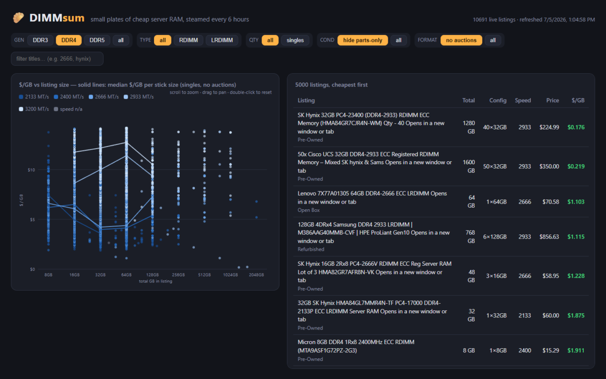
This project exists because I bought 30 sticks of 16GB DDR4-3200 RDIMM for an EPYC build in early April: an r/homelabsales find at $80 a stick, which was a fair price that day. The problem is that “that day” turned out to be the exact top of the market. Buying the top is pretty standard for me. Then the server wouldn’t POST with at least 4 of the sticks installed, and of the 16 that made it in, 4 more start throwing ECC errors the moment I do anything memory-heavy (LLM inferencing, which is of course why I bought them). There are still 6 untested sticks in the box. I knew the going rate; what I couldn’t see was where prices were headed or which sticks would actually work. A price tracker with real sold history fixes at least the first problem.
Beyond my own bad luck, the general problem is that eBay search results for server RAM are a mess. “32GB (2x16GB)” is two 16GB sticks, not one 32GB stick. The same 2666 MT/s speed shows up as DDR4-2666, PC4-21300, PC4-2666V, or just “2666V” depending on the seller’s mood. Lots of 8, lots of 32, single sticks, and “FOR PARTS” boards are all mixed together in the same results. Comparing actual price per gigabyte across all of that by hand is miserable.
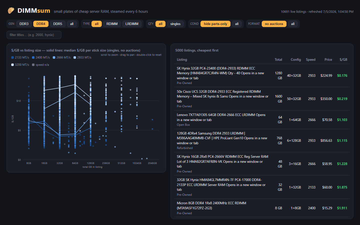
LabGopher solved this years ago for whole servers, and I have wanted the RAM equivalent basically forever. So I built it: DIMMsum, a free site that scrapes eBay every 6 hours, normalizes the listing titles with an LLM, and charts everything as $/GB with median market lines per speed grade.
Welcome to Austin’s Nerdy Things, where we deploy a browser farm and a language model to avoid doing mental math on eBay listings.
My first attempt (2024) was bad
This is actually my second run at scraping eBay. Back in 2024 I wrote a requests + BeautifulSoup scraper that pulled search results through free SOCKS proxies from public proxy lists. It mostly worked, in the sense that it is technically still running on an LXC in my basement, appending to a parse.log that is now 636MB. The proxies were garbage (free proxies are free for a reason), the regex title parsing was wrong constantly, and I never did anything with the data. Classic.
Two things changed since then: eBay got much more aggressive about blocking scrapers, and LLMs got cheap enough to throw at every single listing title. Both of those turned out to matter a lot.
eBay does not want to be scraped (by robots that look like robots)
The 2024 approach is completely dead in 2026. Plain HTTP clients like requests do not even get to say hello anymore – eBay identifies them as robots essentially instantly and serves a 403 or the “Pardon Our Interruption” page. My first attempts with an automated browser got generic eBay error pages on search URLs too, while the exact same URLs worked fine by hand. That one had me confused for a while.
I am going to spare you the play-by-play here, partly because it would be a bot-evasion cookbook published by a site that participates in eBay’s own affiliate program, which seems unwise. The short version: the fix was embarrassingly simple, and it amounted to using a real browser (Playwright driving full Chromium) and having it behave like a polite human instead of a robot in a hurry. Take the path a person would take, slow down, keep the footprint small. No proxies, no stealth plugins, one IP, 3-6 second randomized delays between pages, and eBay has been perfectly happy serving me 240 listings per page ever since – a few hundred page loads a day, total.
The query matrix (or: making the search do half the parsing)
Instead of one broad “ddr4 rdimm” search, DIMMsum runs 51 very specific queries, one per capacity + speed + module type combo:
32gb (2666,pc4-21300,2666v) rdimm -2x16 -4x8 -8x4
The parenthesized part is eBay OR syntax covering the speed synonyms, and the negative terms exclude kit notation so results skew toward true single sticks. The neat part is that each query doubles as a weak label: if a listing was found by the 32GB 2666 RDIMM query but parses out as a 16GB stick, something is off (a lot, a mislabel, or a parse bug), and it gets flagged with a little warning icon in the UI instead of silently polluting the chart.
LLM title parsing for $0.09 per thousand listings
Here is a real title from the database:
2048GB 128x16GB DDR3 PC3L-10600R ECC Reg Server Memory RAM
That is 128 sticks of 16GB low-voltage DDR3-1333 RDIMM. My 2024 regex parser had no chance. The domain rules are genuinely fiddly: a PC3L prefix means low voltage, but a trailing L on the PC number (PC3-14900L) means LRDIMM, and both can appear in the same token. Kit notation states the total first. “LOT” without a count does not mean quantity greater than one. Part numbers are more authoritative than the title text around them.
Rather than encoding all that in regex, every title goes through DeepSeek (deepseek-v4-flash, their cheap model) with a system prompt full of those domain rules, returning structured JSON validated by a pydantic schema:
Titles are batched 25 per API call with an index round-trip check so a misaligned response fails loudly instead of assigning specs to the wrong listings. Against a hand-labeled fixture set it scored 97.4% field accuracy on the first eval run, and the misses were fields that only existed encoded inside part numbers (a future deterministic PN-decode layer will catch those).
The economics are the part that still makes me smile. At roughly $0.09 per 1,000 titles, the total LLM bill for parsing every listing DIMMsum has ever seen is about two dollars. This pipeline was not possible on a hobby budget three years ago; now it is basically free.
The plumbing
Everything lands in Postgres on my Proxmox cluster (one VM for the scraper + web app, one for the database). A systemd timer scrapes every 6 hours, and each run records a price snapshot per listing, which means DIMMsum builds its own price history for every item it tracks. The web side is FastAPI plus one vanilla JavaScript file. No framework. The whole site is a scatter chart, a table, and some server-rendered spec pages.
Current state of the database after a few days of running:
Metric
Count
RAM listings tracked
10,697
Price snapshots
104,475
Search queries per run
51
Scrape frequency
every 6 hours
LLM parse cost, lifetime
~$2
Claude (Fable 5, via Claude Code) wrote most of this code with me over a few evenings. The architecture arguments were real arguments and it lost some of them, but I will happily credit it with the claim-column work queue pattern that lets me run parallel parse workers against Postgres without them stepping on each other.
Sold prices (the part I am most excited about)
Active listing prices tell you what sellers are asking. Sold prices tell you what buyers actually paid, and those are very different numbers on eBay.
I assumed for months that scraping sold/completed listings was off the table and never actually tested it. Turns out the same polite-human browsing approach handles the sold/completed view just fine, and eBay hands you sold prices with dates, 240 per page. I was wrong for months for no reason. Test your assumptions, folks.
So as of this week DIMMsum also harvests sold listings weekly into their own table. The first sweep pulled in over 8,000 real sales, and the sold history goes back further than the ~90 days I expected (most of the usable volume reaches back to late 2025). That data is going to power a monthly “state of the used RAM market” report: median $/GB by SKU, month over month, from real transactions. The June data already shows 8GB DDR4-2133 RDIMMs sliding from $3.50/GB in April to $3.12 in June, and that is exactly the kind of thing I want a monthly email about.
There is a signup box at the bottom of dimmsum.com for exactly that report. One email a month, actual data, no other nonsense.
Disclosure and what’s next
The site is monetized with eBay Partner Network affiliate links: if you click through and buy, eBay pays a commission. That is the entire business model. Free site, no ads, no accounts, and the full disclosure lives in the footer.
Next up: the monthly sold-price report, a storage version (same idea, $/TB for used enterprise SSDs and HDDs, already in progress as a separate project), and a part-number decode table to squeeze out the last few percent of parse accuracy.
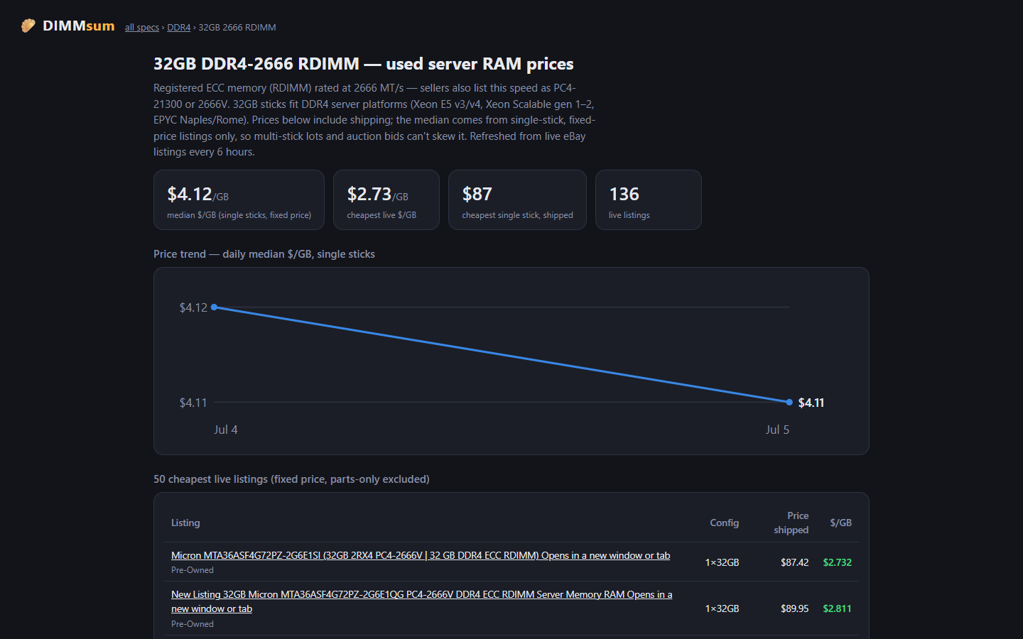
Go find some cheap RDIMMs at dimmsum.com. My benchmark SKU (32GB DDR4-2666 RDIMM singles) has a median around $132 a stick right now with the floor meaningfully below that, and now I get to watch the market instead of refreshing eBay searches like an animal.
A $20 eBay purchase from two years ago just demolished all of that.
The Hardware: Telecom Surplus for Pocket Change
The key piece is an Oscilloquartz OSA-5401 – a GPS-disciplined PTP grandmaster clock in an SFP form factor. These things were designed to plug into telecom switches and provide IEEE 1588 Precision Time Protocol timing for cellular networks. They have a built-in GPS receiver, an OCXO (oven-controlled crystal oscillator), and an FPGA that handles hardware PTP timestamping. New, they cost thousands of dollars. On eBay, a handful of decommissioned units went for $20. Now they’re unavailable. If they do appear (rarely), they’re $300-500.
I first spotted these on a ServeTheHome forum thread back in 2024. Someone found a batch on eBay for $20 each and I jumped on one. The firmware doesn’t include the NTP server feature from the spec sheet (that requires a license), but it spews PTP multicast frames on power-up – and that turns out to be all you need. I posted the first working PTP+chrony config in that thread, which others used as a starting point.
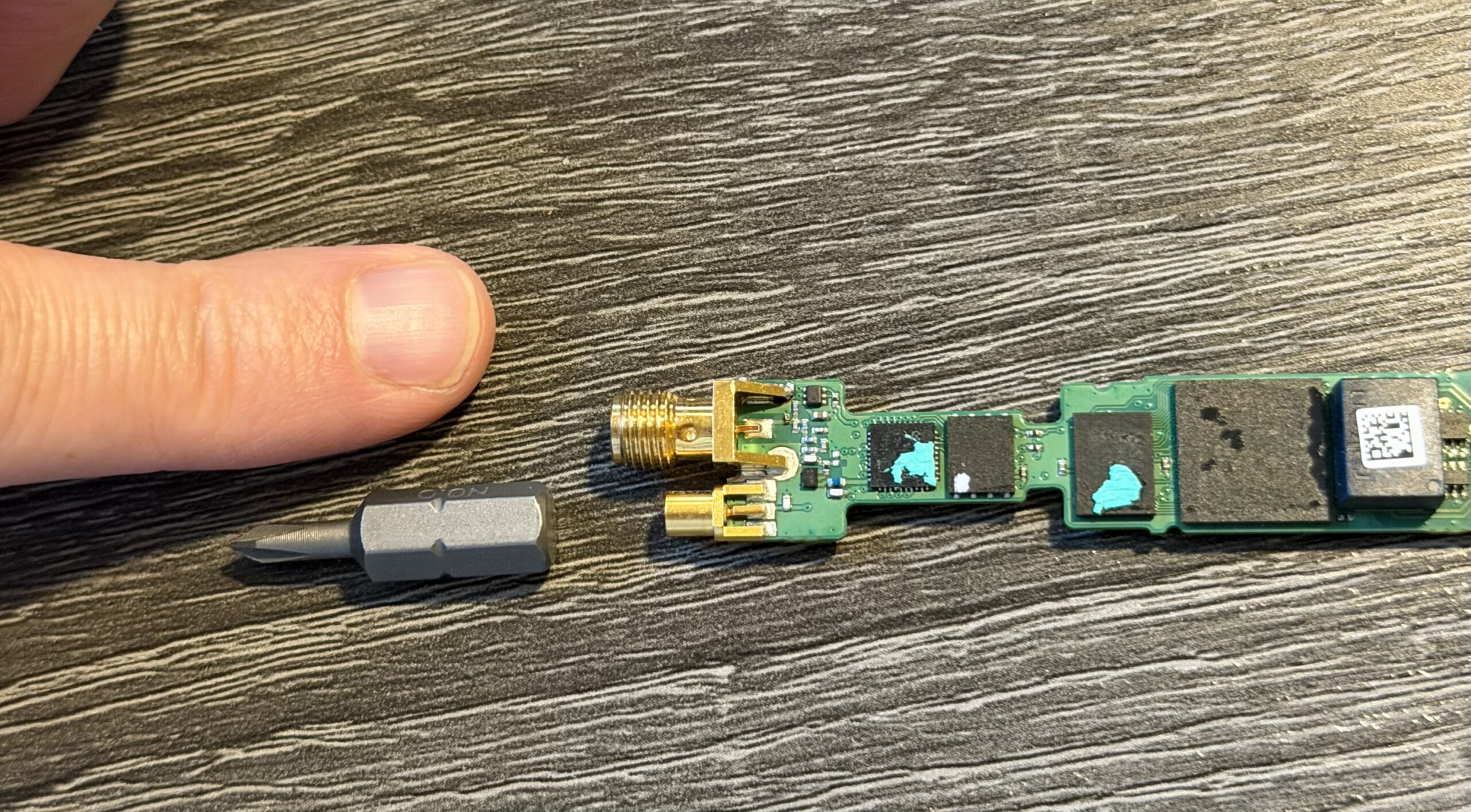
Mine was flaky from the start – the antenna would intermittently disconnect. I reported in the thread that “wiggling the module helped,” which in retrospect should have been a bigger clue. When I finally pulled the board out of the SFP housing, I found the GNSS SMA connector had broken loose from the PCB – probably cracked during decommissioning. A few minutes with a soldering iron fixed that, and it’s been rock solid since. Here’s the board with the resoldered connector, screwdriver bit for scale:
OSA-5401 PCB with resoldered GNSS SMA connector, screwdriver bit for scale
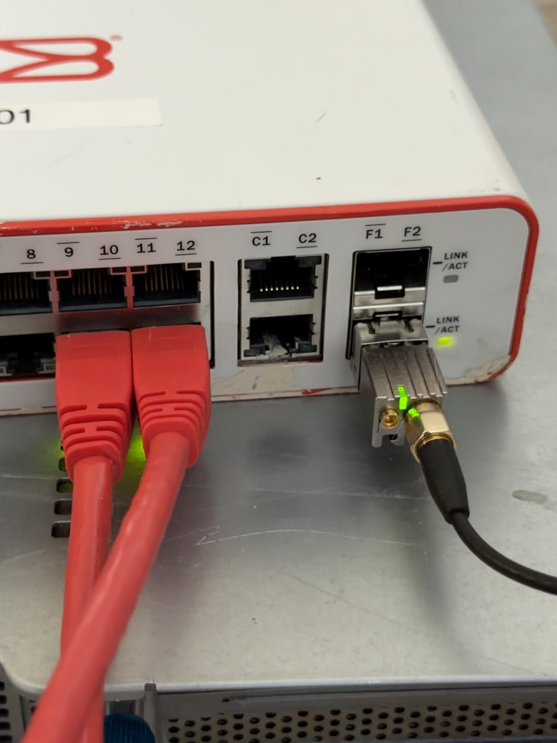
And installed in port F2 of a Brocade ICX6430-C12 switch, GPS antenna connected:
OSA-5401 installed in a Brocade ICX6430-C12 SFP port with GPS antenna
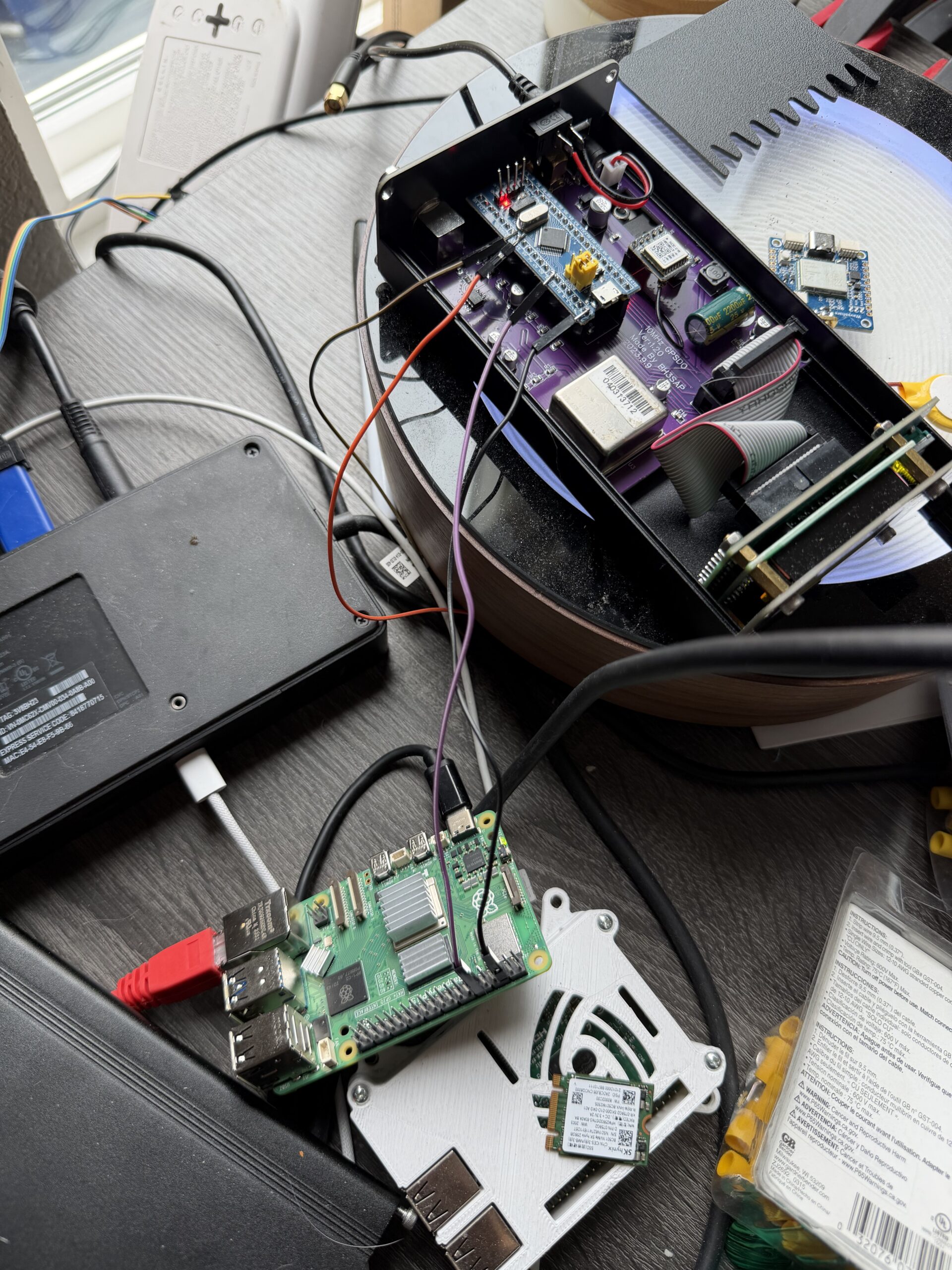
I also have a BH3SAP GPSDO that I picked up for about $70 on eBay – one of those Chinese units with an OX256B OCXO and an STM32 Blue Pill microcontroller. There’s a great thread on EEVBlog about these. I soldered some jumper wires to the MCU PPS output and connected it to GPIO 18 on my Raspberry Pi 5. I’ve been running custom firmware on it (based on fredzo’s gpsdo-fw) with some modifications for telemetry and flywheel display.
The whole mess wired together – GPSDO PPS jumper wires running to the Pi 5’s GPIO header:
GPSDO connected to Raspberry Pi 5 via PPS jumper wires
The Raspberry Pi 5 has hardware timestamping on its Ethernet NIC, which gives it a /dev/ptp0 PTP hardware clock (PHC). This is critical – without hardware timestamping, PTP is no better than NTP. The Pi 5’s Ethernet controller supports it natively.
Here’s the setup:
OSA-5401 ($29) – GPS-disciplined PTP grandmaster, plugged into an SFP port on my network switch
BH3SAP GPSDO (~$70) – GPS-disciplined OCXO, PPS output wired to Pi 5 GPIO
Raspberry Pi 5 – running ptp4l (for PTP) and chronyd (for everything else)
Total cost of timing hardware: ~$100
The Software Stack
The timing chain has two hops:
ptp4l receives PTP sync messages from the OSA-5401 over Ethernet and disciplines the Pi’s PTP hardware clock (/dev/ptp0)
chrony reads the hardware clock as a refclock and disciplines the system clock
The chrony refclock configuration for PTP (/etc/chrony/conf.d/ptp-osa.conf):
# OSA-5401 via ptp4l -> PHC0
# ptp4l disciplines /dev/ptp0 to PTP timescale (TAI)
# tai lets chrony apply the current TAI-UTC offset from its leap second table
refclock PHC /dev/ptp0 refid PTP dpoll -4 poll 0 filter 5 precision 1e-9 tai
A few things worth noting:
tai tells chrony the PHC is on TAI timescale and to automatically apply the current TAI-UTC offset (currently 37 seconds). This is better than hardcoding offset -37 because it auto-updates if a leap second is ever announced again.
dpoll -4 means chrony reads the PHC 16 times per second. I initially had this at dpoll 0 (once per second), but a tcpdump revealed the OSA-5401 is actually sending PTP sync messages at 16 Hz, not 1 Hz. So there’s fresh data to read.
filter 5 takes the median of 5 consecutive reads, rejecting outliers.
precision 1e-9 tells chrony the refclock is accurate to 1 nanosecond, which tightens the error bounds that chrony uses in source selection.
The Bug: Why Chrony Refused to Use the Better Source
When I first got this all running, I had both PPS (from the GPSDO) and PTP (from the OSA-5401) configured as refclocks. The GPSDO had lost GPS lock overnight and had been flywheeling for about 12 hours. PTP was clearly the better source – lower jitter, independent GPS reference. But chrony stubbornly stayed on PPS.
PPS was selected (*) and PTP was marked x – “may be in error.” But PTP wasn’t in error. The GPSDO had drifted 59 microseconds during 12 hours of flywheel, and chrony was faithfully following it off a cliff.
That trust flag is nuclear. It tells chrony: “this source is always correct – never classify it as a falseticker.” Combined with prefer, chrony would choose PPS no matter how much every other source disagreed with it. Three sources (PTP, pi-ntp, pfsense) all agreed the system clock was off by ~59 μs, but chrony trusted PPS absolutely and marked PTP as suspicious instead.
The fix was simple: remove trust. And after some more testing, remove prefer too. Let chrony’s selection algorithm do its job. As soon as I did that:
PTP immediately took over. PPS correctly demoted to - (valid but not selected), showing +59 μs offset – the accumulated GPSDO flywheel drift.
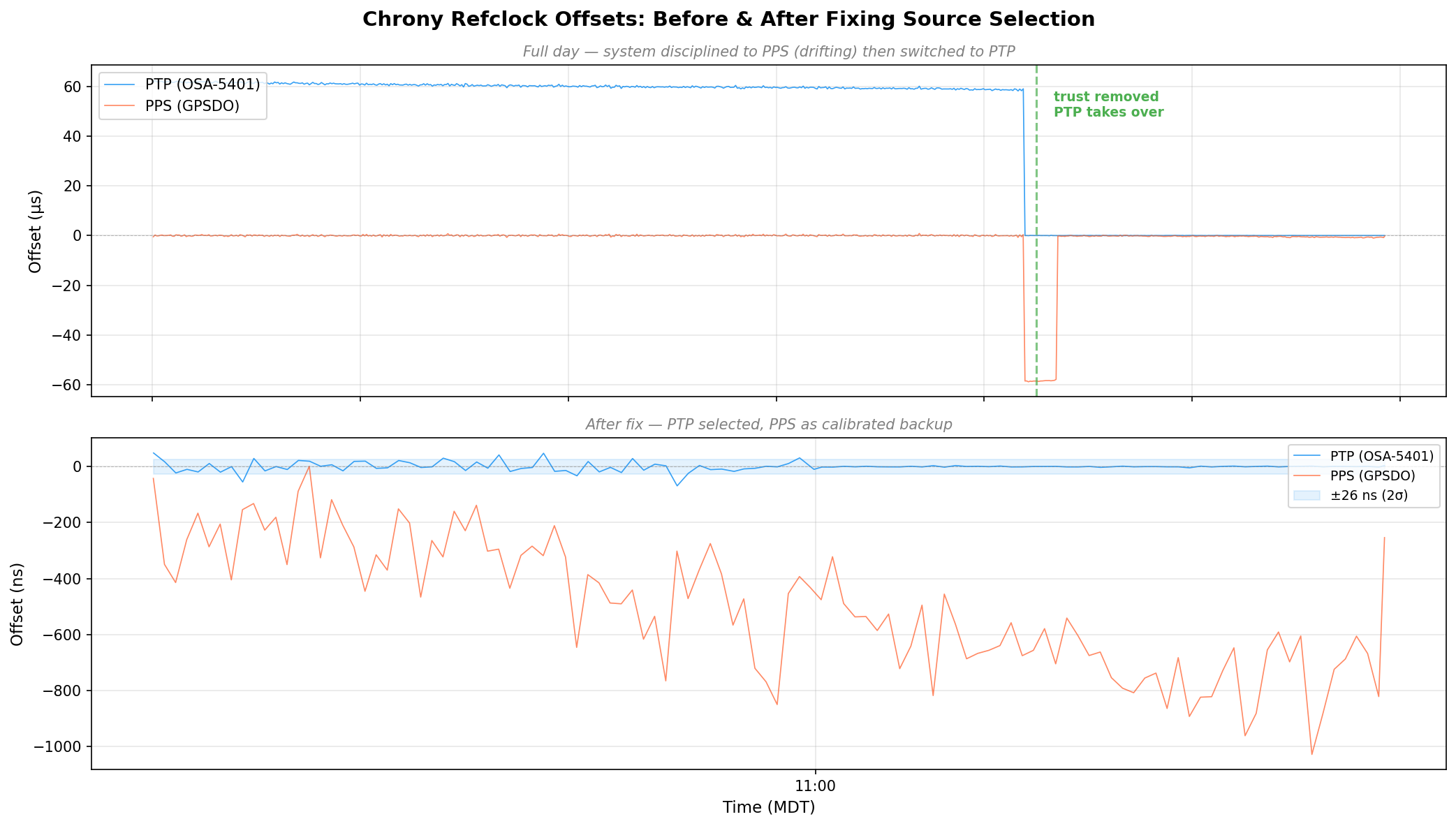
Here’s the full day of refclock data. The top panel is in microseconds – you can see PTP sitting at +60 μs the whole morning because the system clock was following the drifting GPSDO. Then the fix lands around 08:30 MDT and everything snaps into place. The bottom panel zooms into the post-fix period in nanoseconds:
Chrony refclock offsets before and after fixing source selection – PTP drops from 60μs to near-zero
Discovering the 58.3 Microsecond MCU Bias
Once the GPSDO regained GPS lock, I expected PPS to converge back toward PTP. It didn’t. It settled at a rock-solid +58 μs offset with 474 ns standard deviation. Locked, stable, just… late.
The BH3SAP GPSDO doesn’t pass the GPS module’s PPS signal directly to the output. It goes through the STM32 microcontroller – GPIO interrupt, some processing, then the MCU asserts the output pin. And traverses a jumper wire with questionable soldering. That path adds latency (and a not very clean edge). With PTP as ground truth, I could now measure exactly how much.
I pulled 500 samples from chrony’s refclock log and crunched the numbers:
Stat
Value
Mean
-58.319 μs
Median
-58.372 μs
Std Dev
787 ns
P5–P95
-59.2 to -57.4 μs
Range
9.8 μs peak-to-peak
A consistent 58.3 microsecond delay. Sub-microsecond jitter – the MCU interrupt path is deterministic, just slow. The fix is a static offset in the chrony config:
PPS went from +58 μs to +425 ns. The two sources now agree to within a microsecond, and PPS is a legitimate backup if PTP ever drops.
The Results: ±26 Nanoseconds
After tuning the PTP refclock parameters (dpoll -4, poll 0, filter 5), here are the final numbers:
But first, here’s the big picture. This is 36 hours of chrony’s tracking offset – the actual error between the system clock and whatever reference chrony was using at the time:
System clock offset over 36 hours – PPS scattered at ±200 ns, then PTP collapses it to a thin line
The orange scatter is the GPSDO’s PPS running chrony for a day and a half – ±200 ns on a good minute, ±400 ns on a bad one. The green dashed line is the moment I removed trust and PTP took over. The purple line is when I cranked the polling rate to 16 Hz. After that, the data is a flat line at zero on this scale.
ptp4l (OSA-5401 → Pi hardware clock):
Metric
Value
RMS offset
11.8 ns
Max offset
17 ns
Path delay
3,160 ns
chrony (Pi hardware clock → system clock):
Metric
Value
Std Dev
5 ns
RMS offset
4 ns
Frequency skew
0.002 ppm
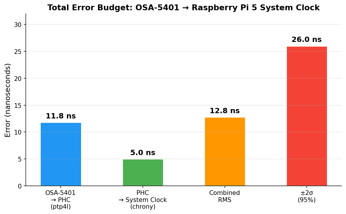
Combined error budget (root sum of squares):
Layer
Error
OSA-5401 → PHC (ptp4l)
11.8 ns
PHC → system clock (chrony)
5.0 ns
Combined RMS
12.8 ns
±2σ (95% confidence)
±26 ns
For comparison, my Pi 3B NTP server that’s been running for years:
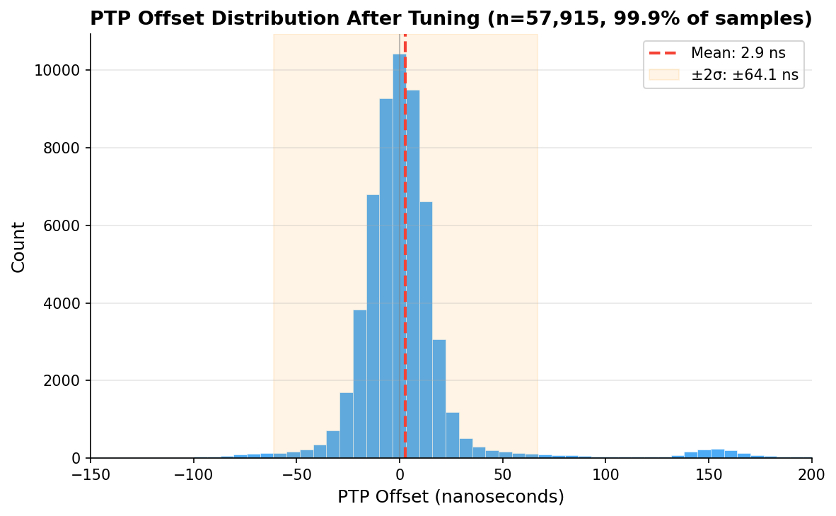
And here’s the distribution of 57,915 PTP offset samples after tuning. Mean of 2.9 ns, tight Gaussian centered right on zero:
PTP offset histogram after tuning – 57,915 samples, mean 2.9 ns
Checking Our Work: What Does the Raw Data Actually Say?
Those numbers above come from what the servos report. ptp4l prints a 1 Hz RMS summary. chrony’s sourcestats shows the standard deviation of its filtered, averaged output. Both are honest numbers, but they’re the numbers after each servo has done its best to smooth things out. What does the raw measurement data look like?
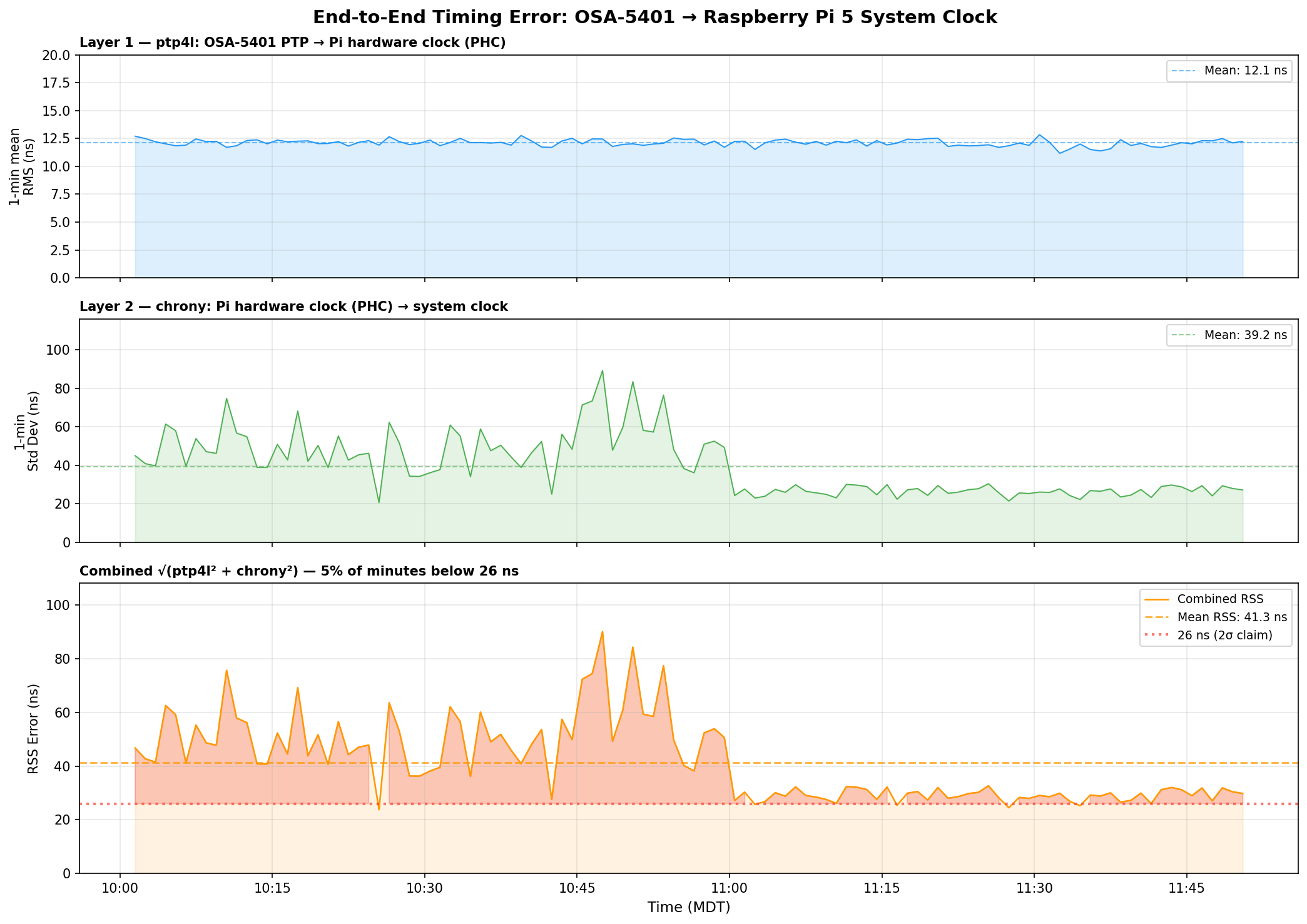
I pulled 110 minutes of overlapping data – ptp4l’s 1 Hz journal summaries and chrony’s 16 Hz raw refclock offset log – and computed 1-minute rolling statistics for each layer, then combined them as root sum of squares:
End-to-end timing error analysis – ptp4l at 12 ns, chrony raw jitter at 39 ns, combined RSS at 41 ns
Three things jump out:
ptp4l is the stable one. Layer 1 (OSA-5401 → PHC) sits at 12.1 ns mean RMS and barely moves. The FPGA doing the hardware timestamping in the OSA-5401 earns its keep here – there’s just not much noise to begin with.
chrony’s raw readings are noisier than its filtered output suggests. The 16 Hz PHC reads have a 39 ns mean standard deviation per minute, with spikes up to 90 ns. But chrony’s sourcestats reports 5 ns – because the median-of-5 filter and the PI servo smooth that out before it touches the system clock. Both numbers are real; they measure different things.
The honest combined number is ±40–50 ns typical, not ±26 ns. The ±26 ns figure from chrony’s tracking output reflects the post-filter error – what the system clock actually experiences after chrony has done its smoothing. The raw measurement chain has more jitter than that. You can see the combined RSS settling toward 27–30 ns in the last hour as the servo tightened, but 40 ns is a fairer typical value.
Even at ±50 ns, that’s still 4× better than the Pi 3B’s ±200 ns. And the trend in the last hour suggests it keeps improving as chrony accumulates more data and tightens its frequency estimate.
GPSDO Flywheel Testing
With the PTP source providing a known-good reference, I can now characterize the GPSDO’s holdover performance. I unplugged the GPSDO’s GPS antenna and let it flywheel on its OCXO. Early results after the first hour showed drift still buried in the noise floor – under 100 ns/hr. The OX256B OCXO in this $70 unit might actually be decent. I’m collecting data for a longer run and will update this post (or write a follow-up) with the full holdover curve.
The dream setup is adding a DS18B20 temperature sensor directly to the OCXO case so I can correlate thermal drift with the oscillator’s frequency offset. That would let me separate temperature-driven drift from aging – but that’s a project for another weekend.
The Journey: Five Years, Six Orders of Magnitude
Year
Post
Method
Accuracy
2021
USB GPS NTP
NTP over USB serial
~1 ms
2021
GPS PPS NTP
GPIO PPS + chrony
~1 μs
2025
Revisiting in 2025
Tuned chrony + Pi 3B
~200 ns
2025
Thermal management
CPU temp stabilization
~86→16 ns RMS
2026
This post
PTP + OSA-5401
±26 ns
From a $12 USB GPS dongle to a $29 telecom SFP module. From milliseconds to nanoseconds. The total cost of the timing hardware in my current setup is about $100, and it’s achieving accuracy that used to require five-figure test equipment.
The next step down would be sub-nanosecond, and that requires White Rabbit – dedicated hardware, specialized SFP transceivers, and budgets measured in tens of thousands. For commodity Ethernet and general-purpose Linux, ±26 nanoseconds is pretty much the floor.
I think I’m done. (For now.) At least, that’s what I told my wife.
Configs for Reference
PTP refclock (/etc/chrony/conf.d/ptp-osa.conf)
# OSA-5401 via ptp4l -> PHC0
# ptp4l disciplines /dev/ptp0 to PTP timescale (TAI)
# tai lets chrony apply the current TAI-UTC offset from its leap second table
refclock PHC /dev/ptp0 refid PTP dpoll -4 poll 0 filter 5 precision 1e-9 tai
PPS refclock (/etc/chrony/conf.d/pps-gpsdo.conf)
# GPSDO 1 Hz PPS on GPIO 18
# dpoll 0 = read every pulse (1 Hz)
# filter 3 = median of 3 samples (odd count for true median)
# poll 2 = 4s loop update (2^2=4 >= filter 3)
# offset = MCU PPS delay compensation (58.3us measured against PTP)
refclock PPS /dev/pps0 refid PPS dpoll 0 poll 2 filter 3 precision 1e-7 offset 0.0000583

# Accurate LAN NTP server - coarse time for PPS second identification
server 10.98.1.198 iburst minpoll 4 maxpoll 6
The hwtimestamp * line enables hardware timestamping on all interfaces, and leapsectz right/UTC is required for the tai refclock option to work correctly.
Disclosure: When you click on links to various merchants in this post and make a purchase, this can result in this site earning a commission. Affiliate programs and affiliations include, but are not limited to, the eBay Partner Network.
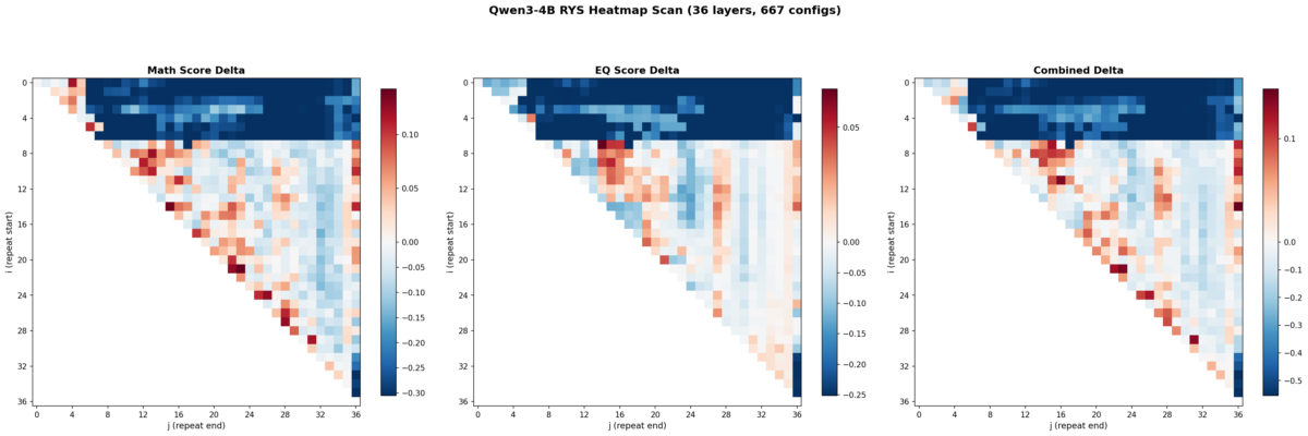
Math delta (left), EQ delta (center), and combined delta (right) across all 667 (i,j) layer duplication configs. The three-phase encode/reason/decode anatomy is clearly visible at 4B scale.
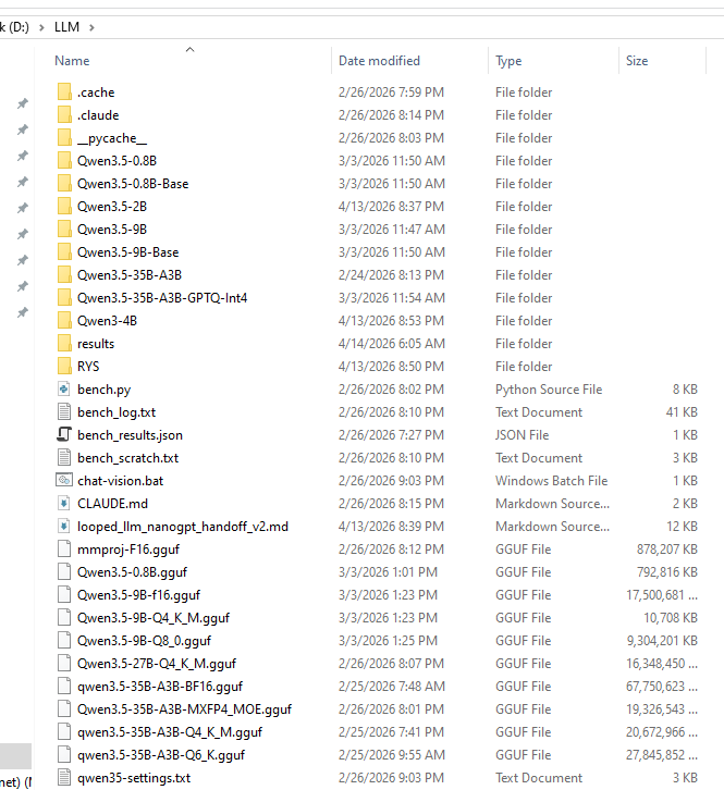
I’ve been messing around with local LLMs on my 3090 for a while now — I have a growing collection of Qwen models on D:\LLM that I probably should be embarrassed about. A few weeks ago I stumbled across David Noel Ng’s LLM Neuroanatomy blog posts, where he showed that you can take a pretrained transformer and literally just re-run some of its middle layers a second time at inference, no retraining needed, and get meaningfully better outputs.
The D:\LLM folder. I should probably be embarrassed about this.
The idea is wild: the model’s weights don’t change. You just tell it “hey, run layers 15 through 21 again” and the hidden state gets another pass through those same weights. Ng showed this working on Qwen3.5-27B (a 64-layer model) with up to +15.6% improvement on combined math and emotional reasoning benchmarks.
Naturally, I wanted to know if this works on smaller models too. Welcome to Austin’s Nerdy Things, where we perform brain surgery on 4-billion-parameter language models to make them think twice.
Background: What Is RYS?
Ng’s technique is called RYS and the core concept is surprisingly simple. A normal transformer forward pass goes:
Process input through layers 0, 1, 2, …, N-1 sequentially
Done
With RYS, you pick a contiguous block in the middle — layers i through j-1 — and after the model finishes layer j-1, you jump back and re-execute layers i through N-1. Those middle layers run twice on the evolving hidden state.
The reason this can work is that transformer layers aren’t all doing the same thing. Ng’s work showed models have a recognizable three-phase anatomy:
Early layers (~0-15% depth): Encoding. Converting tokens into contextualized representations. Repeating these produces garbage — the model tries to re-encode already-encoded stuff.
Middle layers (~20-60% depth): Reasoning. The actual thinking. Repeating these is like giving the model extra time to work through the problem.
Late layers (~70-100% depth): Decoding. Converting internal representations back into token predictions. Repeating these also produces garbage.
Ng found the sweet spot consistently in the middle, and his RYS repo provides all the tooling to test this — layer duplication wrappers, benchmark probe sets, the whole thing.
But his experiments were on a 27B model with 64 layers. I wanted to know: does this three-phase anatomy even exist at 4B scale? Can you exploit it on consumer hardware?
The Setup
Model: Qwen3-4B. I picked this one specifically because it’s a pure dense transformer (36 layers, 2560 hidden dim, GQA with 32 Q / 8 KV heads, RoPE, BF16). The Qwen3.5-2B has hybrid linear/full attention which would complicate things, and Qwen3-4B is in the same model family as Ng’s 27B target, which makes cross-scale comparison cleaner.
Hardware: My trusty RTX 3090 (24 GB VRAM). The model takes about 8.1 GB at baseline, which leaves plenty of room for the KV cache overhead from layer duplication.
Benchmarks: I used Ng’s probe sets from the RYS repo:
Math-16: 16 hard math questions (square roots, cube roots, big multiplications) requiring single-integer answers. Scored with digit-level partial credit. No chain-of-thought allowed. Greedy decoding, 64 max new tokens.
EQ-16: 16 EQ-Bench scenarios — complex social dialogues where the model predicts 4 emotion intensities on a 0-10 scale. Max 256 new tokens.
I used /no_think to disable Qwen3’s thinking mode so we’re measuring raw single-pass capability, and greedy decoding (do_sample=False), which I verified is perfectly deterministic across 5 runs on the same input. No need for multi-run variance testing.
The sweep: All 667 valid (i, j) configurations for a 36-layer model, including baseline (0, 0). Every config runs all 32 probe questions. I added early stopping that triggers if the first 2 math probes both produce garbage (saves about 30% of wall time on broken configs). The scanner saves results to JSON after every single config — resume-friendly for when Windows decides it’s update time.
Total sweep time: about 9 hours on a single 3090. Claude helped me write the scanner script (with me providing the architecture decisions and Ng’s RYS library doing the heavy lifting on layer manipulation).
Baseline Scores
Before messing with anything, Qwen3-4B scores:
Probe
Score
Math-16
0.305
EQ-16
0.749
Combined
1.054
The math score looks low, but these are genuinely hard problems (like “what is the cube root of 1019330085047 times 31?”) and the scorer gives partial credit for getting digits right. The EQ score is actually solid — Qwen3-4B is pretty decent at predicting emotional dynamics even without chain-of-thought.
The Heatmaps
Here’s where it gets fun. I swept all 667 configs and plotted the results as heatmaps. Each cell is one (i, j) configuration. Red means improvement over baseline. Blue means degradation. The x-axis is j (where the repeated block ends) and the y-axis is i (where it starts).
Left: math delta. Center: EQ delta. Right: combined delta. Red = improvement, blue = degradation. 667 configs, 36 layers.
Three things jumped out immediately.
1. The three-phase anatomy is clearly present at 4B scale
The top-left corner (early layers duplicated with wide spans) is deep blue — that’s the encoding zone. The bottom-right corner (late layers) is also blue — that’s the decoding zone. The productive region runs diagonally through the middle. This is exactly the encode / reason / decode structure Ng found at 27B.
Layers 0-6 are the encoding wall. Repeat anything starting before layer 5 with a wide span and the model outputs garbage. Layers 30+ are decoding territory — also garbage if you repeat there. The productive zone lives between layers ~5 and ~27, spanning roughly 60% of the model.
2. Math and EQ have different hot zones
This was something I wasn’t expecting. The math heatmap shows gains across a broad band from mid-stack to upper layers. The EQ heatmap’s gains concentrate in a tighter region around layers 7-16. The combined heatmap shows three distinct hot zones:
Zone A (layers 7-15, ~19-42% depth): Strong EQ gains, moderate math
Zone B (layers 15-20, ~42-56% depth): Balanced improvement on both
Zone C (layers 21-27, ~58-75% depth): Strong math gains, EQ roughly neutral
So the model’s “emotional processing” lives slightly earlier in the stack than its “mathematical processing.” That’s a cool finding — different kinds of reasoning occupy different layer ranges even in a small model.
3. The encoding wall is a cliff, not a slope
The transition from “productive duplication” to “catastrophic failure” happens over 1-2 layers. Layer 5 duplication helps. Layer 3 duplication tanks the model. There’s basically no gradient — it’s a cliff edge. Ng observed something similar at 27B but it’s even more pronounced at 4B scale.
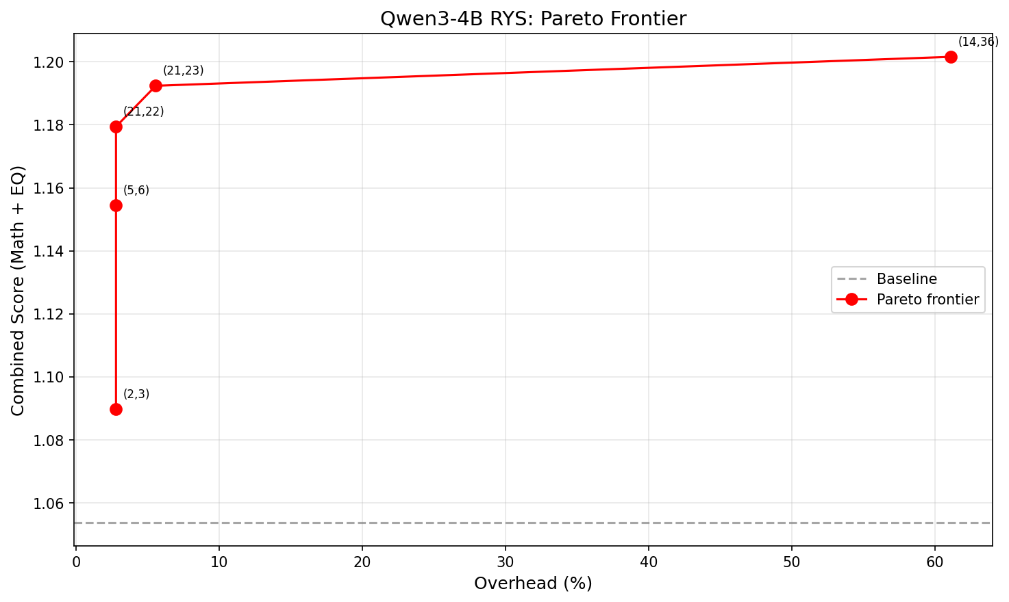
The Pareto Frontier
Not all improvements are worth the extra latency. Each extra layer traversal costs time. The practical question is: how much bang per buck?
X-axis: overhead (%). Y-axis: combined score. The curve is sharply concave — almost all the benefit comes from the first 1-2 extra layers.
Size
Config (i,j)
Extra layers
Overhead
Combined
Improvement
XS
(2,3)
1
2.8%
1.090
+3.4%
S
(5,6)
1
2.8%
1.154
+9.6%
M
(21,22)
1
2.8%
1.179
+11.9%
L
(21,23)
2
5.6%
1.192
+13.2%
XL
(14,36)
22
61.1%
1.202
+14.0%
The winner is (21,22): just repeat layer 21 once. That’s +11.9% combined improvement at 2.8% latency overhead. One single extra layer forward pass. That’s it.
Going from 1 extra layer to 2 buys another 1.3 percentage points. Going from 2 extra layers to 22 — literally 10x the overhead — buys only 0.8 more. The returns collapse fast. Look at that Pareto chart — the curve is basically flat after the first couple of points.
Single-Layer Repeats: The 4B Surprise
This is where things get really interesting, and where the results diverge most from Ng’s 27B findings.
Ng reported that single-layer repeats at 27B “almost never help.” You need to duplicate a contiguous block of at least 2-3 layers to see meaningful improvement at that scale.
At 4B? 14 out of 35 single-layer repeats beat baseline. Here are the top performers:
Layer
Config
Combined delta
21
(21,22)
+0.126
5
(5,6)
+0.101
24
(24,25)
+0.100
26
(26,27)
+0.073
19
(19,20)
+0.071
22
(22,23)
+0.063
20
(20,21)
+0.057
17
(17,18)
+0.049
Layers 5 and 17-26 — nearly the entire mid-to-late stack — all produce meaningful gains when repeated individually. That’s a wide, diffuse productive zone spanning about 60% of the model.
My interpretation: smaller models have less specialized layers. At 27B with 64 layers, each layer does something specific enough that repeating just one doesn’t help much — you need a coherent block. At 4B with 36 layers, individual layers carry more general-purpose reasoning capacity. A single extra pass through one of them is already enough to bump quality.
This is arguably the most practically useful finding from the whole experiment. For small models, even the simplest possible intervention works.
How This Compares to Ng’s 27B Results
Property
Qwen3-4B (36 layers)
Qwen3.5-27B (64 layers)
Three-phase anatomy
Yes, clearly visible
Yes
Encoding wall
Layers 0-6 (~0-17%)
~first 15%
Best single-layer
(21,22) = +11.9%
Rarely productive
Best absolute
(14,36) = +14.0% at 61% overhead
~+15.6% at ~15.6% overhead
Best efficiency
(21,22) = +11.9% at 2.8% overhead
Layer 33 = +1.5%
Productive single layers
14/35 (40%)
Rare
Efficiency curve shape
Sharply concave
Roughly linear to ~10 layers
The biggest difference is the shape of the efficiency curve. At 27B, adding more repeated layers gives roughly linear improvement up to about 10 extra layers — there’s a real reason to invest in multi-layer duplication. At 4B, the curve is sharply concave. Almost all the benefit comes from the very first extra layer. After that, you’re paying a lot of overhead for very little gain.
This makes intuitive sense. A bigger model has more specialized layers where repetition compounds — each one contributes something distinct. A smaller model gets most of its benefit from a single extra pass through its most general-purpose reasoning layer, and additional passes hit diminishing returns because those layers are doing similar work.
What This Means If You Want to Use It
If you’re deploying a small dense model and want better reasoning at minimal cost:
Find the model’s “layer 21.” Run a quick single-layer sweep on your target model. It takes minutes per config.
Repeat that one layer. At 2.8% latency overhead, this is basically free.
Don’t over-invest in multi-layer duplication at small scale. The second extra layer buys way less than the first.
For framework implementers: this is a ~10-line change to a model’s forward pass. No weight changes, no retraining, no meaningful VRAM increase. It should be a first-class inference option in llama.cpp, vLLM, ExLlama, etc.
Caveats
I want to be upfront about what this doesn’t prove:
One model, one family. These results are Qwen3-4B specific. The three-phase anatomy probably generalizes (Ng showed it on multiple architectures), but the exact layer numbers won’t. Every model needs its own sweep.
Small probe sets. 16 math + 16 EQ questions. Enough for relative ordering of configs, but the absolute scores have meaningful variance. Validate on larger benchmarks before deploying.
Greedy decoding only. Sampling might interact differently with layer duplication. I haven’t tested that.
No multi-block compositions. Ng’s beam search finds configs that repeat two different blocks (e.g., layers 30-34 AND 43-45). I only tested single contiguous blocks. The multi-block space at 4B is unexplored.
RoPE positions aren’t adjusted. The model sees the same position IDs on the repeated pass. This works empirically but the theoretical interaction is unclear.
Reproducing This
Everything runs on a single 3090 (or any 24GB+ GPU):
The scanner loads the model once, pre-tokenizes all probes, then iterates through configs. Each config wraps the base model with a layer-index remapping (no weight copies, just pointer rearrangement), runs all probes greedy, scores, and saves. Resume works by checking which config keys already exist in the results JSON.
What’s Next
A few obvious follow-ups I’m thinking about:
Multi-block beam search at 4B. Does combining layers 5-6 and 21-22 compound the gains?
Cross-scale comparison. Run the same sweep on Qwen3.5-2B (hybrid attention), Qwen3.5-9B, maybe a non-Qwen model. See how the efficiency curve changes with scale.
Train-time loop exposure. Train a small model where specific layers are looped during training, compare with inference-time-only duplication.
Integration with inference frameworks. llama.cpp, vLLM, and ExLlama already manage layer weights — adding a “repeat layer N” flag should be pretty straightforward.
The broader takeaway is that transformer layers aren’t interchangeable. They have structure, and that structure is legible even at small scale. You can exploit it at inference time with zero retraining, and the cost is basically nothing.
Layer 21 thinks twice. The model gets smarter. That’s the whole trick.
I’ve been building SkySpottr, an AR app overlaying aircraft information on your phone’s screen, using your device’s location, orientation, and incoming aircraft data (ADS-B) to predict where planes should appear on screen, then uses a YOLO model to lock onto the actual aircraft and refine the overlay. YOLOv8 worked great for this… until I actually read the license.
Welcome to Austin’s Nerdy Things, where we train from scratch entire neural networks to avoid talking to lawyers.
The Problem with Ultralytics
YOLOvWhatver is excellent. Fast, accurate, easy to use, great documentation. But Ultralytics licenses it under AGPL-3.0, which means if you use it in a product, you either need to open-source your entire application or pay for a commercial license. For a side project AR app that I might eventually monetize? That’s a hard pass.
Enter YOLOX from Megvii (recommended by either ChatGPT or Claude, can’t remember which, as an alternative). MIT licensed. Do whatever you want with it. The catch? You have to train your own models from scratch instead of using Ultralytics’ pretrained weights and easy fine-tuning pipeline. I have since learned there are some pretrained models. I didn’t use them.
So training from scratch is what I did. Over a few late nights in December 2025, I went from zero YOLOX experience to running custom-trained aircraft detection models in my iOS app. Here’s how it went.
The Setup
Hardware: RTX 3090 on my Windows machine, COCO2017 dataset on network storage (which turned out to be totally fine for training speed), and way too many terminal windows open.
I started with the official YOLOX repo and the aircraft class from COCO2017. The dataset has about 3,000 training images with airplanes, which is modest but enough to get started.
The first training run failed immediately because I forgot to install YOLOX as a package. Classic. Then it failed again because I was importing a class that didn’t exist in the version I had. Claude (who was helping me through this, and hallucinated said class) apologized and fixed the import. We got there eventually.
Training Configs: Nano, Tiny, Small, and “Nanoish”
YOLOX has a nice inheritance-based config system. You create a Python file, inherit from a base experiment class, and override what you want. I ended up with four different configs:
yolox_nano_aircraft.py – The smallest. 0.9M params, 1.6 GFLOPs. Runs on anything.
yolox_tiny_aircraft.py – Slightly bigger with larger input size for small object detection.
yolox_small_aircraft.py – 5M params, 26 GFLOPs. The “serious” model.
yolox_nanoish_aircraft.py – My attempt at something between nano and tiny.
The “nanoish” config was my own creation where I tried to find a sweet spot. I bumped the width multiplier from 0.25 to 0.33 and… immediately got a channel mismatch error because 0.33 doesn’t divide evenly into the architecture. Turns out you can’t just pick arbitrary numbers. I am a noob at these things. Lesson learned.
After some back-and-forth, I settled on a config with 0.3125 width (which is 0.25 \* 1.25, mathematically clean) and 512×512 input. This gave me roughly 1.2M params – bigger than nano, smaller than tiny, and it actually worked.
Here’s the small model config – the one that ended up in production. The key decisions are width = 0.50 (2x wider than nano for better feature extraction), 640×640 input for small object detection, and full mosaic + mixup augmentation:
class Exp(MyExp):
    def __init__(self):
        super(Exp, self).__init__()

        # Model config - YOLOX-Small architecture
        self.num_classes = 1  # Single class: airplane
        self.depth = 0.33
        self.width = 0.50  # 2x wider than nano for better feature extraction

        # Input/output config - larger input helps small object detection
        self.input_size = (640, 640)
        self.test_size = (640, 640)
        self.multiscale_range = 5  # Training will vary from 480-800

        # Data augmentation
        self.mosaic_prob = 1.0
        self.mosaic_scale = (0.1, 2.0)
        self.enable_mixup = True
        self.mixup_prob = 1.0
        self.flip_prob = 0.5
        self.hsv_prob = 1.0

        # Training config
        self.warmup_epochs = 5
        self.max_epoch = 400
        self.no_aug_epochs = 100
        self.basic_lr_per_img = 0.01 / 64.0
        self.scheduler = "yoloxwarmcos"

    def get_model(self):
        from yolox.models import YOLOX, YOLOPAFPN, YOLOXHead

        in_channels = [256, 512, 1024]
        # Small uses standard convolutions (no depthwise)
        backbone = YOLOPAFPN(self.depth, self.width, in_channels=in_channels, act=self.act)
        head = YOLOXHead(self.num_classes, self.width, in_channels=in_channels, act=self.act)
        self.model = YOLOX(backbone, head)
        return self.model
And the nanoish config for comparison – note the depthwise=True and the width of 0.3125 (5/16) that I landed on after the channel mismatch debacle:
class Exp(MyExp):
    def __init__(self):
        super(Exp, self).__init__()

        self.num_classes = 1
        self.depth = 0.33
        self.width = 0.3125  # 5/16 - halfway between nano (0.25) and tiny (0.375)

        self.input_size = (512, 512)
        self.test_size = (512, 512)

        # Lighter augmentation than small - this model is meant to be fast
        self.mosaic_prob = 0.5
        self.mosaic_scale = (0.5, 1.5)
        self.enable_mixup = False

    def get_model(self):
        from yolox.models import YOLOX, YOLOPAFPN, YOLOXHead

        in_channels = [256, 512, 1024]
        backbone = YOLOPAFPN(self.depth, self.width, in_channels=in_channels,
                             act=self.act, depthwise=True)  # Depthwise = lighter
        head = YOLOXHead(self.num_classes, self.width, in_channels=in_channels,
                         act=self.act, depthwise=True)
        self.model = YOLOX(backbone, head)
        return self.model
The -c yolox_s.pth loads YOLOX’s pretrained COCO weights as a starting point (transfer learning). The -d 1 is one GPU, -b 16 is batch size 16 (about 8GB VRAM on the 3090 with fp16), and --fp16 enables mixed precision training.
The Small Object Problem
Here’s the thing about aircraft detection for an AR app: planes at cruise altitude look tiny. A 747-8 at 37,000 feet is maybe 20-30 pixels on your phone screen if you’re lucky, even with the 4x optical zoom of the newest iPhones (8x for the 12MP weird zoom mode). Standard YOLO models are tuned for reasonable-sized objects, not specks in the sky. The COCO dataset has aircraft that are reasonably sized, like when you’re sitting at your gate at an airport and take a picture of the aircraft 100 ft in front of you.
My first results were underwhelming. The nano model was detecting larger aircraft okay but completely missing anything at altitude. The evaluation metrics looked like this:
AP for airplane = 0.234
AR for small objects = 0.089
Not great. The model was basically only catching aircraft on approach or takeoff.
For the small config, I made some changes to help with tiny objects:
Increased input resolution to 640×640 (more pixels = more detail for small objects)
Enabled full mosaic and mixup augmentation (helps the model see varied object scales)
Switched from depthwise to regular convolutions (more capacity)
(I’ll be honest, I was leaning heavily on Claude for the ML-specific tuning decisions here)
This pushed the model to 26 GFLOPs though, which had me worried about phone performance.
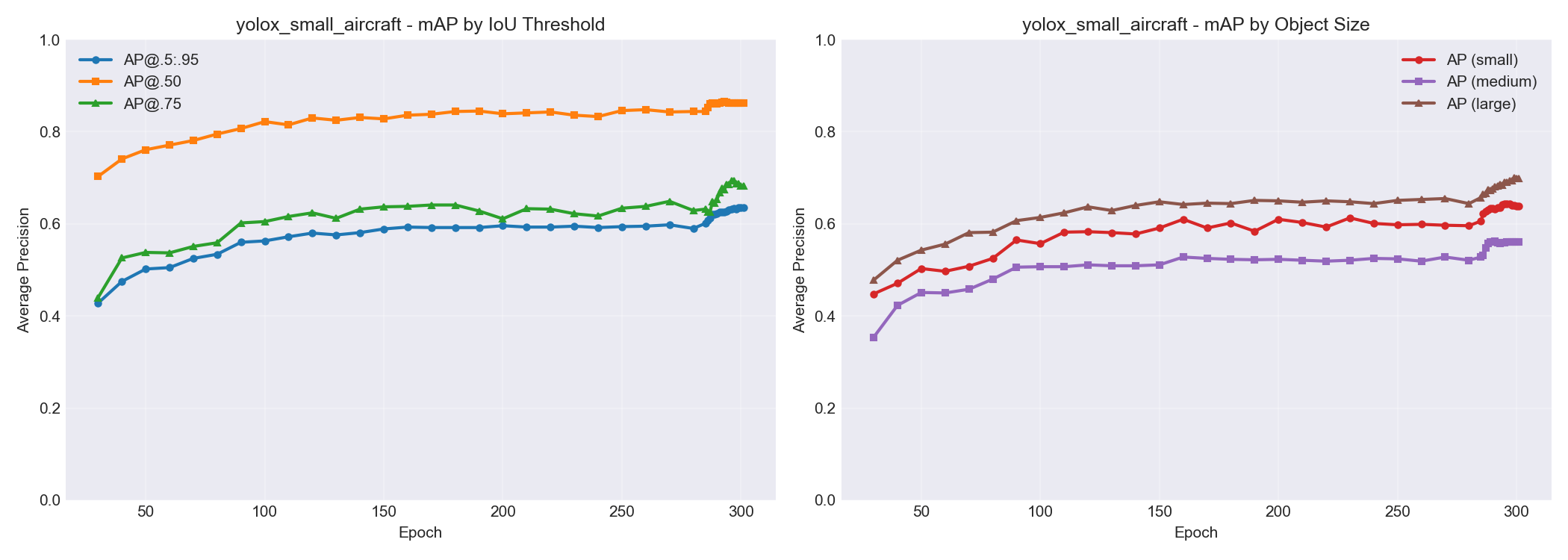
Here’s what the small model’s accuracy looked like broken down by object size. You can see AP for small objects climbing from ~0.45 to ~0.65 over training, while large objects hit ~0.70. Progress, but small objects remain the hardest category – which tracks with the whole “specks in the sky” problem.
Will This Actually Run on a Phone?
The whole point of this exercise was to run inference on an iPhone. So here is some napkin math:
Model
GFLOPs
Estimated Phone Inference
Nano
1.6
~15ms, smooth 30fps easy
Nanoish
3.2
~25ms, still good
Small
26
~80ms, might be sluggish
YOLOv8n (for reference)
8.7
~27ms
My app was already running YOLOv8n at 15fps with plenty of headroom. So theoretically even the small model should work, but nano/nanoish would leave more room for everything else the app needs to do.
The plan: train everything, compare accuracy, quantize for deployment, and see what actually works in practice.
Training Results (And a Rookie Mistake)
After letting things run overnight (300 epochs takes a while even on a 3090), here’s what I got:
The nanoish model at epoch 100 was already showing 94% detection rate on test images, beating the fully-trained nano model. And it wasn’t even done training yet.
Quick benchmark on 50 COCO test images with aircraft (RTX 3090 GPU inference – not identical to phone, but close enough for the smaller models to be representative):
Model
Detection Rate
Avg Detections/Image
Avg Inference (ms)
FPS
YOLOv8n
58.6%
0.82
33.6
29.7
YOLOX nano
74.3%
1.04
14.0
71.4
YOLOX nanoish
81.4%
1.14
15.0
66.9
YOLOX tiny
91.4%
1.28
16.5
60.7
YOLOX small
92.9%
1.30
17.4
57.4
Ground Truth
–
1.40
–
–
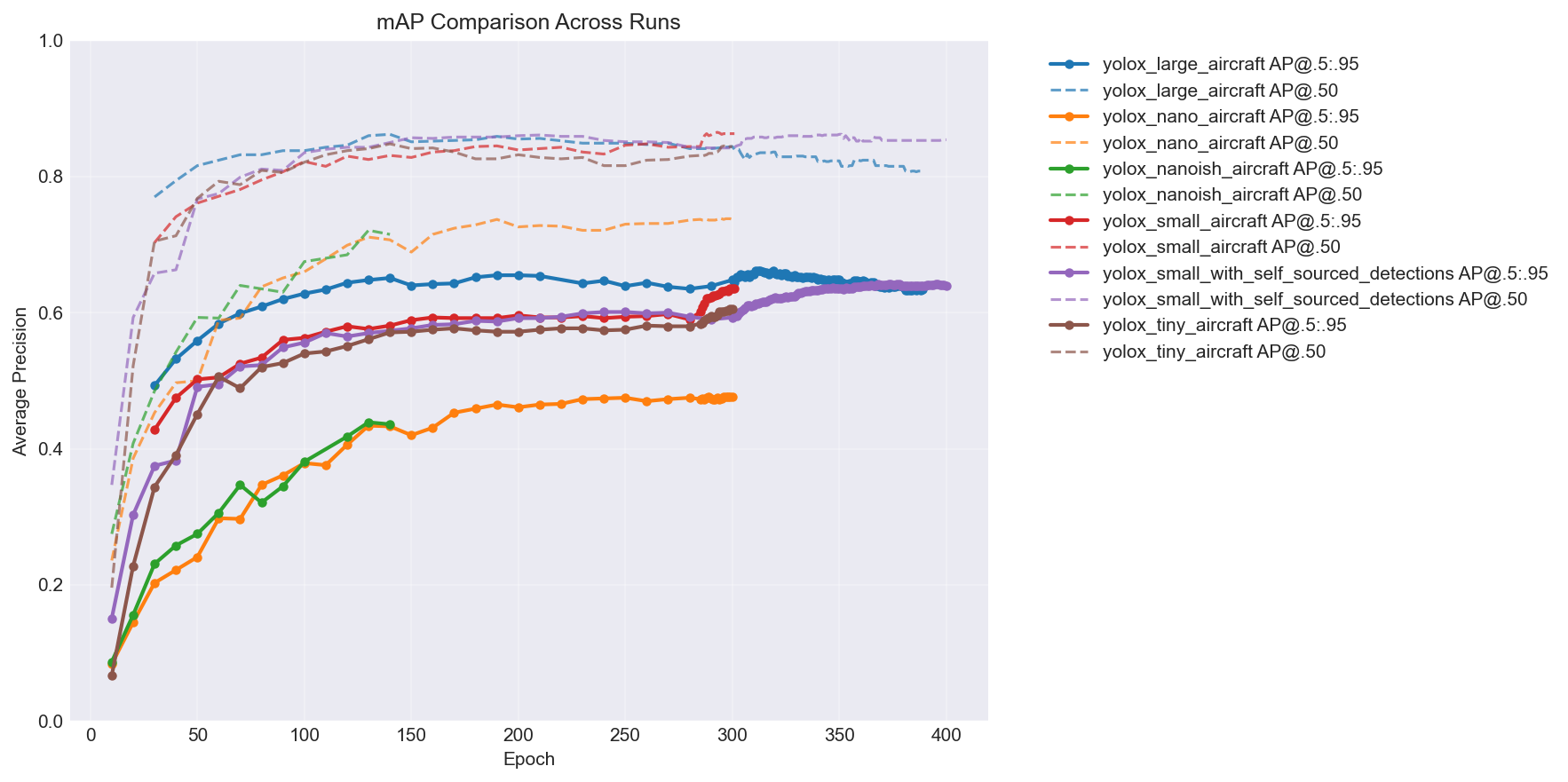
YOLOv8n getting beaten by every single YOLOX variant while also being slower was… not what I expected. Here’s the mAP comparison across all the models over training – you can see the hierarchy pretty clearly:
The big takeaway: more capacity = better accuracy, but with diminishing returns. The jump from nano to nanoish is huge, nanoish to small is solid, and tiny lands somewhere in between depending on the epoch. (You’ll notice two extra lines in the chart – a large model and a self-sourced variant. I kept training after this post’s story ends. More on the self-sourced pipeline later. You can also see the large model is clearly overfitting past epoch ~315 – loss keeps decreasing but mAP starts dropping. My first time overfitting a model.)
The nanoish model hit a nice sweet spot. Faster than YOLOv8n, better small object detection than pure nano, and still lightweight enough for mobile.
And here is the output from my plot_training.py script:
But there was a problem I didn’t notice until later: my training dataset had zero images without aircraft in them. Every single training image contained at least one airplane. This is… not ideal if you want your model to learn what an airplane isn’t. More on that shortly.
How It Actually Works in the App
Before I get to results, here’s what the ML is actually doing in SkySpottr. The app combines multiple data sources to track aircraft:
ADS-B data tells us where aircraft are in 3D space (lat, lon, altitude)
Device GPS and orientation tell us where the phone is and which way it’s pointing
Physics-based prediction places aircraft overlays on screen based on all the above
That prediction is usually pretty good, but phone sensors drift and aircraft positions are slightly delayed. So the overlays can be off by a couple degrees. This is where YOLO comes in.
The app runs the model on each camera frame looking for aircraft. When it finds one within a threshold distance of where the physics engine predicted an aircraft should be, it “snaps” the overlay to the actual detected position. The UI shows an orange circle around the aircraft and marks it as “SkySpottd” – confirmed via machine learning.
I call this “ML snap” mode. It’s the difference between “there’s probably a plane somewhere around here” and “that specific bright dot is definitely the aircraft.”
The model runs continuously on device, which is why inference time matters so much. Even at 15fps cap, that’s still 15 inference cycles per second competing with everything else the app needs to do (sensor fusion, WebSocket data, AR rendering, etc.). Early on I was seeing 130%+ CPU usage on my iPhone, which is not great for battery life. Every millisecond saved on inference is a win.
Getting YOLOX into CoreML
One thing the internet doesn’t tell you: YOLOX and Apple’s Vision framework don’t play nice together.
YOLOv8 exports to CoreML with a nice Vision-compatible interface. You hand it an image, it gives you detections. Easy. YOLOX expects different preprocessing – it wants pixel values in the 0-255 range (not normalized 0-1), and the output tensor layout is different.
The conversion pipeline goes PyTorch → TorchScript → CoreML. Here’s the core of it:
import torch
import coremltools as ct
from yolox.models import YOLOX, YOLOPAFPN, YOLOXHead

# Build model (same architecture as training config)
backbone = YOLOPAFPN(depth=0.33, width=0.50, in_channels=[256, 512, 1024], act="silu")
head = YOLOXHead(num_classes=1, width=0.50, in_channels=[256, 512, 1024], act="silu")
model = YOLOX(backbone, head)

# Load trained weights
ckpt = torch.load("yolox_small_best.pth", map_location="cpu", weights_only=False)
model.load_state_dict(ckpt["model"])
model.eval()
model.head.decode_in_inference = True  # Output pixel coords, not raw logits

# Trace and convert
dummy = torch.randn(1, 3, 640, 640)
traced = torch.jit.trace(model, dummy)
mlmodel = ct.convert(
    traced,
    inputs=[ct.TensorType(name="images", shape=(1, 3, 640, 640))],
    outputs=[ct.TensorType(name="output")],
    minimum_deployment_target=ct.target.iOS15,
    convert_to="mlprogram",
)
mlmodel.save("yolox_small_aircraft.mlpackage")
The decode_in_inference = True is crucial — without it, the model outputs raw logits and you’d need to implement the decode head in Swift. With it, the output is [1, N, 6] where 6 is [x_center, y_center, width, height, obj_conf, class_score] in pixel coordinates.
On the Swift side, Claude ended up writing a custom detector that bypasses the Vision framework entirely. Here’s the preprocessing — the part that was hardest to get right:
/// Convert pixel buffer to MLMultiArray [1, 3, H, W] with 0-255 range
private func preprocess(pixelBuffer: CVPixelBuffer) -> MLMultiArray? {
    // GPU-accelerated resize via Core Image
    let ciImage = CIImage(cvPixelBuffer: pixelBuffer)
    let scaleX = CGFloat(inputSize) / ciImage.extent.width
    let scaleY = CGFloat(inputSize) / ciImage.extent.height
    let scaledImage = ciImage.transformed(by: CGAffineTransform(scaleX: scaleX, y: scaleY))

    // Reuse pixel buffer from pool (memory leak fix #1)
    var resizedBuffer: CVPixelBuffer?
    CVPixelBufferPoolCreatePixelBuffer(kCFAllocatorDefault, pool, &resizedBuffer)
    guard let buffer = resizedBuffer else { return nil }
    ciContext.render(scaledImage, to: buffer)

    // Reuse pre-allocated MLMultiArray (memory leak fix #2)
    guard let array = inputArray else { return nil }

    CVPixelBufferLockBaseAddress(buffer, .readOnly)
    defer { CVPixelBufferUnlockBaseAddress(buffer, .readOnly) }

    let bytesPerRow = CVPixelBufferGetBytesPerRow(buffer)
    let pixels = CVPixelBufferGetBaseAddress(buffer)!.assumingMemoryBound(to: UInt8.self)
    let arrayPtr = array.dataPointer.assumingMemoryBound(to: Float.self)
    let channelStride = inputSize * inputSize

    // BGRA → RGB, keep 0-255 range (YOLOX expects unnormalized pixels)
    // Direct pointer access is ~100x faster than MLMultiArray subscript
    for y in 0..<inputSize {
        let rowOffset = y * bytesPerRow
        let yOffset = y * inputSize
        for x in 0..<inputSize {
            let px = rowOffset + x * 4
            let idx = yOffset + x
            arrayPtr[idx] = Float(pixels[px + 2])                      // R
            arrayPtr[channelStride + idx] = Float(pixels[px + 1])      // G
            arrayPtr[2 * channelStride + idx] = Float(pixels[px])      // B
        }
    }
    return array
}
The two key gotchas: (1) BGRA byte order from the camera vs RGB that the model expects, and (2) YOLOX wants raw 0-255 pixel values, not the 0-1 normalized range that most CoreML models expect. If you normalize, everything silently breaks — the model runs, returns garbage, and you spend an evening wondering why.
For deployment, I used CoreML’s INT8 quantization (coremltools.optimize.coreml.linear_quantize_weights). This shrinks the model by about 50% with minimal accuracy loss. The small model went from ~17MB to 8.7MB, and inference time improved slightly.
Real World Results (Round 1)
I exported the nanoish model and got it running in SkySpottr. The good news: it works. The ML snap feature locks onto aircraft, the orange verification circles appear, and inference is fast enough that I don’t notice any lag.
The less good news: false positives. Trees, parts of houses, certain cloud formations – the model occasionally thinks these are aircraft. Remember that rookie mistake about no negative samples? Yeah.
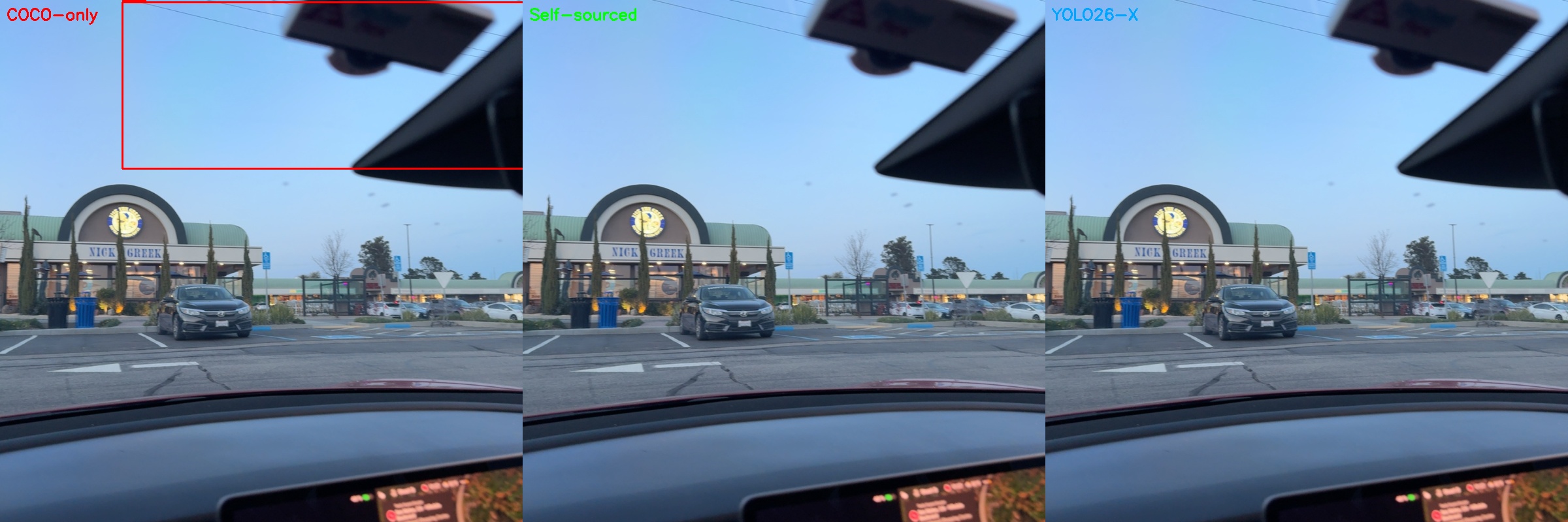
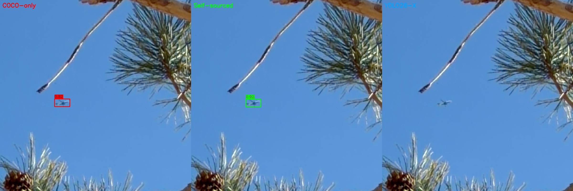
I later set up a 3-way comparison to visualize exactly this kind of failure. The three panels show my COCO-only trained model (red boxes), a later model trained on self-sourced images (green boxes – I’ll explain this pipeline shortly), and YOLO26-X as a ground truth oracle (right panel, no boxes means no detection). The COCO-only model confidently detects an “aircraft” that is… a building. The other two correctly ignore it.
The app handles this gracefully because of the matching threshold. Random false positives in empty sky don’t trigger the snap because there’s no predicted aircraft nearby to match against. But when there’s a tree branch right next to where a plane should be, the model sometimes locks onto the wrong thing.
The even less good news: it still struggles with truly distant aircraft. A plane at 35,000 feet that’s 50+ miles away is basically a single bright pixel. No amount of ML is going to reliably detect that. For those, the app falls back on pure ADS-B prediction, which is usually good enough to get the overlay in the right general area.
But when it works, it works. I’ll show some examples of successful detections in the self-sourced section below.
The Memory Leak Discovery (Fun Debugging Tangent)
While testing the YOLOX integration, I was also trying to get RevenueCat working for subscriptions. Had the app running for about 20 minutes while I debugged the in-app purchase flow. Noticed it was getting sluggish, opened Instruments, and… yikes.
Base memory for the app is around 200MB. After 20 minutes of continuous use, it had climbed to 450MB. Classic memory leak pattern.
The culprit was AI induced, and AI resolved: it was creating a new CVPixelBuffer and MLMultiArray for every single frame. At 15fps, that’s 900 allocations per minute that weren’t getting cleaned up fast enough.
The fix was straightforward – use a CVPixelBufferPool for the resize buffers and pre-allocate a single MLMultiArray that gets reused. Memory now stays flat even after hours of use.
(The RevenueCat thing? I ended up ditching it entirely and going with native StoreKit2. RevenueCat is great, but keeping debug and release builds separate was more hassle than it was worth for a side project. StoreKit2 is actually pretty nice these days if you don’t need the analytics. I’m at ~80 downloads, and not a single purchase. First paid app still needs some fine tuning, clearly, on the whole freemium thing.)
Round 2: Retraining with Negative Samples
After discovering the false positive issue, I went back and retrained. This time I made sure to include images without aircraft – random sky photos, clouds, trees, buildings, just random COCO2017 stuff. The model needs to learn what’s NOT an airplane just as much as what IS one.
Here’s the extraction script that handles the negative sampling. The key insight: you need to explicitly tell the model what empty sky looks like:
def extract_airplane_dataset(split="train", negative_ratio=0.2, seed=42):
    """Extract airplane images from COCO, with negative samples."""
    with open(f"instances_{split}2017.json") as f:
        coco_data = json.load(f)

    # Find all images WITH airplanes
    airplane_image_ids = set()
    for ann in coco_data['annotations']:
        if ann['category_id'] == AIRPLANE_CATEGORY_ID:  # 5 in COCO
            airplane_image_ids.add(ann['image_id'])

    # Find images WITHOUT airplanes for negative sampling
    all_ids = {img['id'] for img in coco_data['images']}
    negative_ids = all_ids - airplane_image_ids

    # Add 20% negative images (no airplanes = teach model what ISN'T a plane)
    num_negatives = int(len(airplane_image_ids) * negative_ratio)
    sampled_negatives = random.sample(list(negative_ids), num_negatives)
    # ... copy images and annotations to output directory
I also switched from nanoish to the small model. The accuracy improvement on distant aircraft was worth the extra compute, and with INT8 quantization the inference time came in at around 5.6ms on an iPhone – way better than my napkin math predicted. Apple’s Neural Engine is impressive.
The final production model: YOLOX-Small, 640×640 input, INT8 quantized, ~8.7MB on disk. It runs at 15fps with plenty of headroom for the rest of the app on my iPhone 17 Pro.
Round 3: Self-Sourced Images and Closing the Loop
So the model works, but it was trained entirely on COCO2017 – airport tarmac photos, stock images, that kind of thing. My app is pointing at the sky from the ground. Those are very different domains.
I added a debug flag to SkySpottr for my phone that saves every camera frame where the model fires a detection. Just flip it on, walk around outside for a while, and the app quietly collects real-world training data. Over a few weeks of casual use, I accumulated about 2,000 images from my phone.
The problem: these images don’t have ground truth labels. I’m not going to sit there and manually draw bounding boxes on 2,000 sky photos. So I used YOLO26-X (Ultralytics’ latest and greatest, which I’m fine using as an offline tool since it never ships in the app) as a teacher model. Run it on all the collected images, take its high-confidence detections as pseudo-labels, convert to COCO annotation format, and now I have a self-sourced dataset to mix in with the original COCO training data.
Here’s the pseudo-labeling pipeline. First, run the teacher model on all collected images:
from ultralytics import YOLO

model = YOLO("yolo26x.pt")  # Big model, accuracy over speed

for img_path in tqdm(image_paths, desc="Processing images"):
    results = model(str(img_path), conf=0.5, verbose=False)
    boxes = results[0].boxes
    airplane_boxes = boxes[boxes.cls == AIRPLANE_CLASS_ID]

    for box in airplane_boxes:
        xyxy = box.xyxy[0].cpu().numpy().tolist()
        x1, y1, x2, y2 = xyxy
        detections.append({
            "bbox_xywh": [x1, y1, x2 - x1, y2 - y1],  # COCO format
            "confidence": float(box.conf[0]),
        })
Then convert those detections to COCO annotation format so YOLOX can train on them:
def convert_to_coco(detections):
    """Convert YOLO26 detections to COCO training format."""
    coco_data = {
        "images": [], "annotations": [],
        "categories": [{"id": 1, "name": "airplane", "supercategory": "vehicle"}],
    }

    for uuid, data in detections.items():
        img_path = Path(data["image_path"])
        width, height = Image.open(img_path).size

        if width > 1024 or height > 1024:  # Skip oversized images
            continue

        coco_data["images"].append({"id": image_id, "file_name": f"{uuid}.jpg",
                                     "width": width, "height": height})

        for det in data["detections"]:
            coco_data["annotations"].append({
                "id": ann_id, "image_id": image_id, "category_id": 1,
                "bbox": det["bbox_xywh"], "area": det["bbox_xywh"][2] * det["bbox_xywh"][3],
                "iscrowd": 0,
            })

    with open("instances_train.json", "w") as f:
        json.dump(coco_data, f)
Finally, combine both datasets in the training config using YOLOX’s ConcatDataset:
Out of 2,000 images, YOLO26-X found aircraft in about 108 of them at a 0.5 confidence threshold – a 1.8% hit rate, which makes sense since most frames are just empty sky between detections. I filtered out anything over 1024px and ended up with a nice supplementary dataset of aircraft-from-the-ground images.
The 3-way comparison images I showed earlier came from this pipeline. Here’s what successful detections look like – the COCO-only model (red), self-sourced model (green), and YOLO26-X (right panel, shown at full resolution so you can see what we’re actually detecting):
That’s maybe 30 pixels of airplane against blue sky, detected with 0.88 and 0.92 confidence by the two YOLOX variants.
And here’s one I particularly like – aircraft spotted through pine tree branches. Real-world conditions, not a clean test image. Both YOLOX models nail it, YOLO26-X misses at this confidence threshold:
And a recent one from February 12, 2026 – a pair of what appear to be F/A-18s over Denver at 4:22 PM MST, captured at 12x zoom. The model picks up both jets at 73-75% confidence, plus the bird in the bottom-right at 77% (a false positive the app filters out via ADS-B matching). Not bad for specks against an overcast sky.
I also trained a full YOLOX-Large model (depth 1.0, width 1.0, 1024×1024 input) on the combined dataset, just to see how far I could push it. Too heavy for phone deployment, but useful for understanding the accuracy ceiling.
Conclusion
Was this worth it to avoid Ultralytics’ licensing? Since it took an afternoon and a couple evenings of vibe-coding, yes, it was not hard to switch. Not just because MIT is cleaner than AGPL, but because I learned a ton about how these models actually work. The Ultralytics ecosystem is so polished that it’s easy to treat it as a black box. Building from YOLOX forced me to understand some of the nuances, the training configs, and the tradeoffs between model size and accuracy.
Plus, I can now say I trained my own object detection model from scratch. That’s worth something at parties. Nerdy parties, anyway.
SkySpottr is live on the App Store if you want to see the model in action – point your phone at the sky and watch it lock onto aircraft in real-time.
The self-sourced pipeline is still running. Every time I use the app with the debug flag on, it collects more training data. The plan is to periodically retrain as the dataset grows – especially now that I’m getting images from different weather conditions, times of day, and altitudes. The COCO-only model was a solid start, but a model trained on actual ground-looking-up images of aircraft at altitude? That’s the endgame.
But there was a problem. Despite having a stable PPS reference, my NTP server’s frequency drift was exhibiting significant variation over time. After months (years) of monitoring the system with Grafana dashboards, I noticed something interesting: the frequency oscillations seemed to correlate with CPU temperature changes. The frequency would drift as the CPU heated up during the day and cooled down at night, even though the PPS reference remained rock-solid.
Like clockwork (no pun intended), I somehow get sucked back into trying to improve my setup every 6-8 weeks. This post is the latest on that never-ending quest.
This post details how I achieved an 81% reduction in frequency variability and 77% reduction in frequency standard deviation through a combination of CPU core pinning and thermal stabilization. Welcome to Austin’s Nerdy Things, where we solve problems that 99.999% of people (and 99% of datacenters) don’t have.
The Problem: Thermal-Induced Timing Jitter
Modern CPUs, including those in Raspberry Pis, use dynamic frequency scaling to save power and manage heat. When the CPU is idle, it runs at a lower frequency (and voltage). When load increases, it scales up. This is great for power efficiency, but terrible for precision timekeeping.
Why? Because timekeeping (with NTP/chronyd/others) relies on a stable system clock to discipline itself against reference sources. If the CPU frequency is constantly changing, the system clock’s tick rate varies, introducing jitter into the timing measurements. Even though my PPS signal was providing a mostly perfect 1-pulse-per-second reference, the CPU’s frequency bouncing around made it harder for chronyd to maintain a stable lock.
But here’s the key insight: the system clock is ultimately derived from a crystal oscillator, and crystal oscillator frequency is temperature-dependent. The oscillator sits on the board near the CPU, and as the CPU heats up and cools down throughout the day, so does the crystal. Even a few degrees of temperature change can shift the oscillator’s frequency by parts per million – exactly what I was seeing in my frequency drift graphs. The CPU frequency scaling was one factor, but the underlying problem was that temperature changes were affecting the crystal oscillator itself. By stabilizing the CPU temperature, I could stabilize the thermal environment for the crystal oscillator, keeping its frequency consistent.
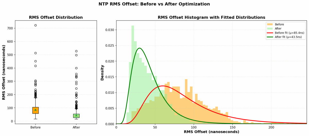
Looking at my Grafana dashboard, I could see the frequency offset wandering over a range of about 1 PPM (parts per million) as the Pi warmed up and cooled down throughout the day. The RMS offset was averaging around 86 nanoseconds, which isn’t terrible (it’s actually really, really, really good), but I knew it could be better.
The Discovery
After staring at graphs for longer than I’d like to admit, I had an idea: what if I could keep the CPU at a constant temperature? If the temperature (and therefore the frequency) stayed stable, maybe the timing would stabilize too.
The solution came in two parts:
1. CPU core isolation – Dedicate CPU 0 exclusively to timing-critical tasks (chronyd and PPS interrupts) 2. Thermal stabilization – Keep the other CPUs busy to maintain a constant temperature, preventing frequency scaling
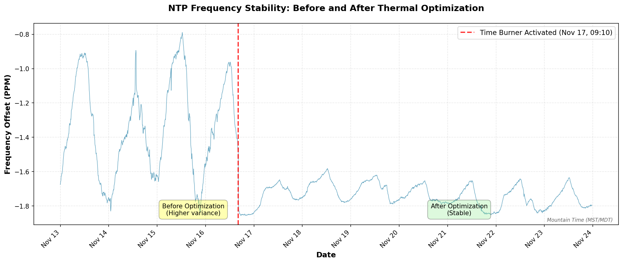
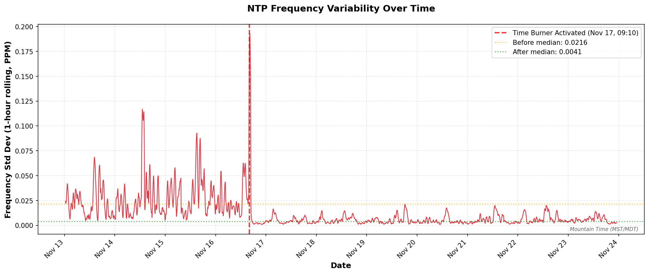
Here’s what happened when I turned on the thermal stabilization system on November 17, 2025 at 09:10 AM:
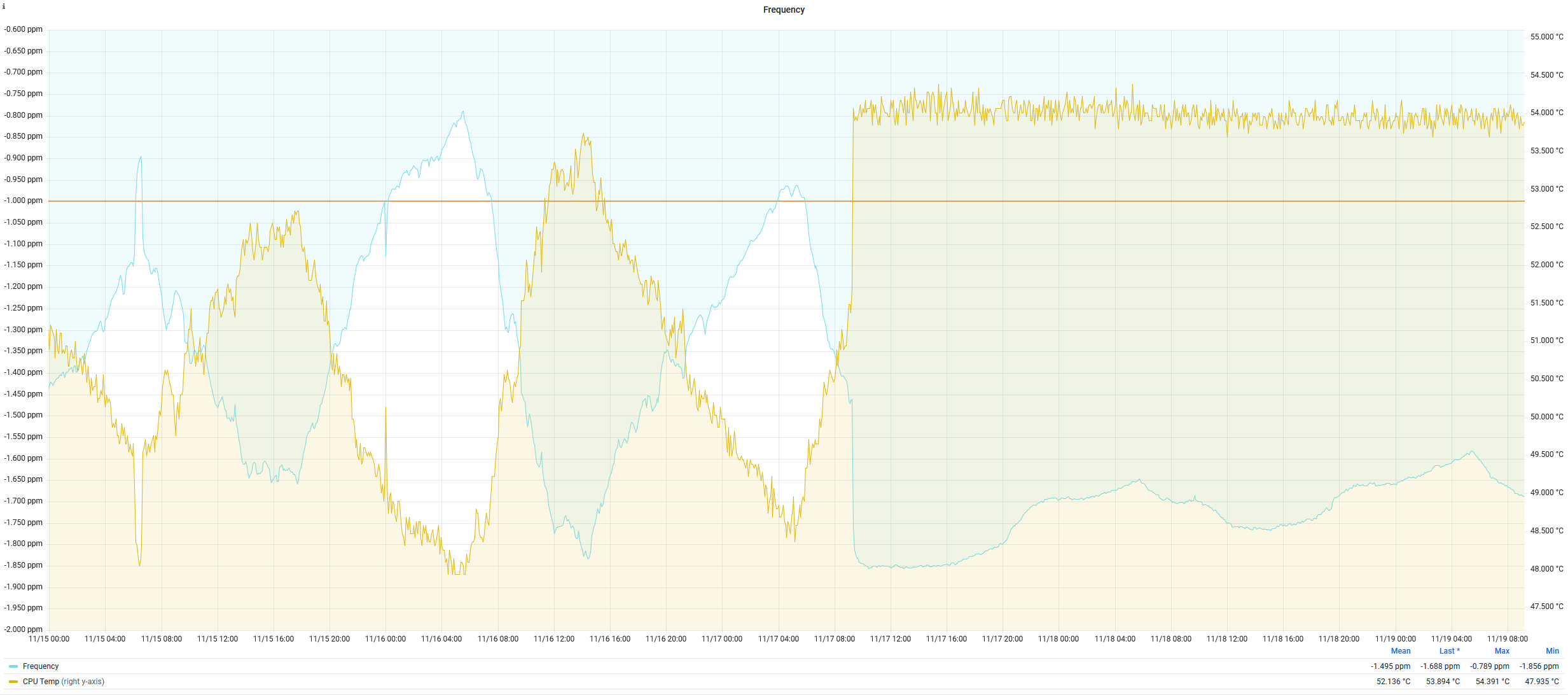
Same ish graph but with CPU temp also plotted:
That vertical red line marks on the first plot when I activated the “time burner” process. Notice how the frequency oscillations immediately dampen and settle into a much tighter band? Let’s dive into how this works.
The Solution Part 1: CPU Core Pinning and Real-Time Priority
The first step is isolating timing-critical operations onto a dedicated CPU core. On a Raspberry Pi (4-core ARM), this means:
CPU 0: Reserved for chronyd and PPS interrupts
CPUs 1-3: Everything else, including our thermal load
I had AI (probably Claude Sonnet 4 ish, maybe 4.5) create a boot optimization script that runs at system startup:
#!/bin/bash
# PPS NTP Server Performance Optimization Script
# Sets CPU affinity, priorities, and performance governor at boot

set -e

echo "Setting up PPS NTP server performance optimizations..."

# Wait for system to be ready
sleep 5

# Set CPU governor to performance mode
echo "Setting CPU governor to performance..."
cpupower frequency-set -g performance

# Pin PPS interrupt to CPU0 (may fail if already pinned, that's OK)
echo "Configuring PPS interrupt affinity..."
echo 1 > /proc/irq/200/smp_affinity 2>/dev/null || echo "PPS IRQ already configured"

# Wait for chronyd to start
echo "Waiting for chronyd to start..."
timeout=30
while [ $timeout -gt 0 ]; do
    chronyd_pid=$(pgrep chronyd 2>/dev/null || echo "")
    if [ -n "$chronyd_pid" ]; then
        echo "Found chronyd PID: $chronyd_pid"
        break
    fi
    sleep 1
    ((timeout--))
done

if [ -z "$chronyd_pid" ]; then
    echo "Warning: chronyd not found after 30 seconds"
else
    # Set chronyd to real-time priority and pin to CPU 0
    echo "Setting chronyd to real-time priority and pinning to CPU 0..."
    chrt -f -p 50 $chronyd_pid
    taskset -cp 0 $chronyd_pid
fi

# Boost ksoftirqd/0 priority
echo "Boosting ksoftirqd/0 priority..."
ksoftirqd_pid=$(ps aux | grep '\[ksoftirqd/0\]' | grep -v grep | awk '{print $2}')
if [ -n "$ksoftirqd_pid" ]; then
    renice -n -10 $ksoftirqd_pid
    echo "ksoftirqd/0 priority boosted (PID: $ksoftirqd_pid)"
else
    echo "Warning: ksoftirqd/0 not found"
fi

echo "PPS NTP optimization complete!"

# Log current status
echo "=== Current Status ==="
echo "CPU Governor: $(cat /sys/devices/system/cpu/cpu0/cpufreq/scaling_governor)"
echo "PPS IRQ Affinity: $(cat /proc/irq/200/effective_affinity_list 2>/dev/null || echo 'not readable')"
if [ -n "$chronyd_pid" ]; then
    echo "chronyd Priority: $(chrt -p $chronyd_pid)"
fi
echo "======================"
What this does:
Performance Governor: Forces all CPUs to run at maximum frequency, disabling frequency scaling
PPS IRQ Pinning: Ensures PPS interrupt (IRQ 200) is handled exclusively by CPU 0
Chronyd Real-Time Priority: Sets chronyd to SCHED_FIFO priority 50, giving it preferential CPU scheduling
Chronyd CPU Affinity: Pins chronyd to CPU 0 using taskset
ksoftirqd Priority Boost: Improves priority of the kernel softirq handler on CPU 0
This script can be added to /etc/rc.local or as a systemd service to run at boot.
The Solution Part 2: PID-Controlled Thermal Stabilization
Setting the performance governor helps, but on a Raspberry Pi, even at max frequency, the CPU temperature will still vary based on ambient conditions and load. Temperature changes affect the CPU’s actual operating frequency due to thermal characteristics of the silicon.
The solution? Keep the CPU at a constant temperature using a PID-controlled thermal load. I call it the “time burner” (inspired by CPU burn-in tools, but with precise temperature control).
As a reminder of what we’re really doing here: we’re maintaining a stable thermal environment for the crystal oscillator. The RPi 3B’s 19.2 MHz oscillator is physically located near the CPU on the Raspberry Pi board, so by actively controlling CPU temperature, we’re indirectly controlling the oscillator’s temperature. Since the oscillator’s frequency is temperature-dependent (this is basic physics of quartz crystals), keeping it at a constant temperature means keeping its frequency stable – which is exactly what we need for precise timekeeping.
Here’s how it works:
Read CPU temperature from /sys/class/thermal/thermal_zone0/temp
PID controller calculates how much CPU time to burn to maintain target temperature (I chose 54°C)
Three worker processes run on CPUs 1, 2, and 3 (avoiding CPU 0)
Each worker alternates between busy-loop (MD5 hashing) and sleeping based on PID output
Temperature stabilizes at the setpoint, preventing thermal drift
Here’s the core implementation (simplified for readability):
#!/usr/bin/env python3
import time
import argparse
import multiprocessing
import hashlib
import os
from collections import deque

class PIDController:
    """Simple PID controller with output clamping and anti-windup."""
    def __init__(self, Kp, Ki, Kd, setpoint, output_limits=(0, 1), sample_time=1.0):
        self.Kp = Kp
        self.Ki = Ki
        self.Kd = Kd
        self.setpoint = setpoint
        self.output_limits = output_limits
        self.sample_time = sample_time
        self._last_time = time.time()
        self._last_error = 0.0
        self._integral = 0.0
        self._last_output = 0.0

    def update(self, measurement):
        """Compute new output of PID based on measurement."""
        now = time.time()
        dt = now - self._last_time

        if dt < self.sample_time:
            return self._last_output

        error = self.setpoint - measurement

        # Proportional
        P = self.Kp * error

        # Integral with anti-windup
        self._integral += error * dt
        I = self.Ki * self._integral

        # Derivative
        derivative = (error - self._last_error) / dt if dt > 0 else 0.0
        D = self.Kd * derivative

        # Combine and clamp
        output = P + I + D
        low, high = self.output_limits
        output = max(low, min(high, output))

        self._last_output = output
        self._last_error = error
        self._last_time = now

        return output

def read_cpu_temperature(path='/sys/class/thermal/thermal_zone0/temp'):
    """Return CPU temperature in Celsius."""
    with open(path, 'r') as f:
        temp_str = f.read().strip()
    return float(temp_str) / 1000.0

def burn_cpu(duration):
    """Busy-loop hashing for 'duration' seconds."""
    end_time = time.time() + duration
    m = hashlib.md5()
    while time.time() < end_time:
        m.update(b"burning-cpu")

def worker_loop(worker_id, cmd_queue, done_queue):
    """
    Worker process:
    - Pins itself to CPUs 1, 2, or 3 (avoiding CPU 0)
    - Burns CPU based on commands from main process
    """
    available_cpus = [1, 2, 3]
    cpu_to_use = available_cpus[worker_id % len(available_cpus)]
    os.sched_setaffinity(0, {cpu_to_use})
    print(f"Worker {worker_id} pinned to CPU {cpu_to_use}")

    while True:
        cmd = cmd_queue.get()
        if cmd is None:
            break

        burn_time, sleep_time = cmd
        burn_cpu(burn_time)
        time.sleep(sleep_time)
        done_queue.put(worker_id)

# Main control loop (simplified)
def main():
    target_temp = 54.0  # degrees Celsius
    control_window = 0.20  # 200ms cycle time

    pid = PIDController(Kp=0.05, Ki=0.02, Kd=0.0,
                        setpoint=target_temp,
                        sample_time=0.18)

    # Start 3 worker processes
    workers = []
    cmd_queues = []
    done_queue = multiprocessing.Queue()

    for i in range(3):
        q = multiprocessing.Queue()
        p = multiprocessing.Process(target=worker_loop, args=(i, q, done_queue))
        p.start()
        workers.append(p)
        cmd_queues.append(q)

    try:
        while True:
            # Measure temperature
            current_temp = read_cpu_temperature()

            # PID control: output is fraction of time to burn (0.0 to 1.0)
            output = pid.update(current_temp)

            # Convert to burn/sleep times
            burn_time = output * control_window
            sleep_time = control_window - burn_time

            # Send command to all workers
            for q in cmd_queues:
                q.put((burn_time, sleep_time))

            # Wait for workers to complete
            for _ in range(3):
                done_queue.get()

            print(f"Temp={current_temp:.2f}C, Output={output:.2f}, "
                  f"Burn={burn_time:.2f}s")

    except KeyboardInterrupt:
        for q in cmd_queues:
            q.put(None)
        for p in workers:
            p.join()

if __name__ == '__main__':
    main()
The full implementation includes a temperature filtering system to smooth out sensor noise and command-line arguments for tuning the PID parameters.
PID Tuning Notes:
Kp=0.05: Proportional gain – responds to current error
Ki=0.02: Integral gain – eliminates steady-state error
Kd=0.0: Derivative gain – set to zero because temperature changes slowly
The target temperature of 54°C was chosen empirically – high enough to keep the CPU from idling down, but low enough to avoid thermal throttling (which starts around 80°C on Raspberry Pi).
The Results: Numbers Don’t Lie
The improvement was immediately visible. Here are the statistics comparing performance before and after the optimization:
A note on ambient conditions: The Raspberry Pi lives in a project enclosure in our master bedroom (chosen for its decent GPS reception and ADS-B coverage for a new aircraft AR overlay app idea I’m working on also running on this Pi). While the time burner maintains the CPU die temperature at 54°C, the enclosure is still subject to ambient temperature swings. Room temperature cycles from a low of 66°F (18.9°C) at 5:15 AM to a peak of 72°F (22.2°C) at 11:30 AM – a 6°F daily swing from our heating schedule. The fact that we see such dramatic frequency stability improvements despite this ambient variation speaks to how effective the thermal control is. The CPU’s active heating overwhelms the environmental changes, maintaining consistent silicon temperature where it matters most.
Frequency Stability
Metric
Before
After
Improvement
Mean RMS Offset
85.44 ns
43.54 ns
49.0% reduction
Median RMS Offset
80.13 ns
37.93 ns
52.7% reduction
The RMS offset is chronyd’s estimate of the timing uncertainty. Cutting this nearly in half means the system is maintaining significantly better time accuracy.
Setup Instructions
Want to replicate this? Here’s the step-by-step process:
Prerequisites
You need a working GPS PPS NTP server setup. If you don’t have one yet, follow my 2025 NTP guide first.
# Verify CPU governor
cat /sys/devices/system/cpu/cpu0/cpufreq/scaling_governor
# Should output: performance

# Check chronyd CPU affinity and priority
ps -eo pid,comm,psr,ni,rtprio | grep chronyd
# Should show psr=0 (CPU 0) and rtprio=50

# Check time burner processes
ps aux | grep time_burner
# Should show 4 processes (1 main + 3 workers)

# Monitor NTP performance
chronyc tracking
Example output from chronyc tracking:
Reference ID    : 50505300 (PPS)
Stratum         : 1
Ref time (UTC)  : Sun Nov 24 16:45:23 2025
System time     : 0.000000038 seconds fast of NTP time
Last offset     : -0.000000012 seconds
RMS offset      : 0.000000035 seconds
Frequency       : 1.685 ppm slow
Residual freq   : -0.001 ppm
Skew            : 0.002 ppm
Root delay      : 0.000000001 seconds
Root dispersion : 0.000010521 seconds
Update interval : 16.0 seconds
Leap status     : Normal
Notice the RMS offset of 35 nanoseconds – this is the kind of accuracy you can achieve with thermal stabilization.
Step 6: Monitor Over Time
(Topic for a future post)
Set up Grafana dashboards to monitor:
Frequency offset (PPM)
RMS offset (nanoseconds)
CPU temperature
System time offset
You’ll see the frequency stabilize within a few hours as the PID controller locks onto the target temperature.
Monitoring and Troubleshooting
Real-Time Monitoring
Watch chronyd tracking in real-time:
watch -n 1 "chronyc tracking"
Check time burner status:
sudo systemctl status time-burner.service
View time burner output:
sudo journalctl -u time-burner.service -f
Common Issues
Temperature overshoots or oscillates:
Adjust PID gains – reduce Kp if oscillating, increase Ki if steady-state error
Try different target temperatures (50-60°C range)
High CPU usage (obviously):
This is intentional – the time burner uses ~90% of 3 cores
Not suitable for Pis running other workloads
Chronyd not pinned to CPU 0:
Check that the optimization script runs after chronyd starts
Adjust the timing in the systemd service dependencies
Trade-offs and Considerations
Let’s be honest about the downsides:
Power Consumption
The time burner keeps 3 cores at ~30% average utilization. My Pi now draws about 3-4W continuously (vs 1-2W idle). Over a year, that’s an extra 15-25 kWh, or about $2-3 in electricity (depending on your rates).
Heat
Running at 54°C means the Pi is warm to the touch. This is well within safe operating temperature (thermal throttling doesn’t start until 80°C), but you might want to ensure adequate ventilation. I added a small heatsink just to be safe.
CPU Resources
You’re dedicating 3 of 4 cores to burning cycles. This is fine for a dedicated NTP server, but not suitable if you’re running other services on the same Pi. That said, I am also running the feeder to my new ADS-B aircraft visualization app on it. My readsb instance regularly gets to 1200 msg/s with 200+ aircraft.
Is It Worth It?
For 99.999% of use cases: absolutely not.
Most applications don’t need better than millisecond accuracy, let alone the 35-nanosecond RMS offset I’m achieving. Even for distributed systems, microsecond-level accuracy is typically overkill.
When this might make sense:
Precision timing applications (scientific instrumentation, radio astronomy)
Distributed systems research requiring tight clock synchronization
Network testing where timing precision affects results
Because you can (the best reason for any homelab project)
For me, this falls squarely in the “because you can” category. I had the monitoring infrastructure in place, noticed the thermal correlation, and couldn’t resist solving the problem. Plus, I learned a lot about PID control, CPU thermal characteristics, and Linux real-time scheduling.
Future Improvements
Some ideas I’m considering:
Adaptive PID Tuning
The current PID gains are hand-tuned for a specific ambient temperature range. The fairly low P value is to avoid spikes when some load on the Pi kicks up the temp. The I is a balance to keep long term “burn” relatively consistent. Implementing an auto-tuning algorithm (like Ziegler-Nichols) or adaptive PID could handle seasonal temperature variations better.
Hardware Thermal Control
Instead of software thermal control, I could add an actively cooled heatsink with PWM fan control. This might achieve similar temperature stability while using less power overall.
Oven-Controlled Crystal Oscillator (OCXO)
For the ultimate in frequency stability, replacing the Pi’s crystal with a temperature-controlled OCXO would eliminate thermal drift at the source. This is how professional timing equipment works. I do have a BH3SAP GPSDO sitting next to me (subject to a future post)… Then again, I’m the person who just wrote 4000 words about optimizing a $50 time server, so who am I kidding?
Conclusions
Through a combination of CPU core isolation and PID-controlled thermal stabilization, I achieved:
81% reduction in frequency variability
77% reduction in frequency standard deviation
74% reduction in frequency range
49% reduction in RMS offset
The system now maintains 38-nanosecond median RMS offset from the GPS PPS reference, with frequency drift that’s barely detectable in the noise. The CPU runs at a constant 54°C, and in steady state, the frequency offset stays within a tight ±0.14 PPM band (compared to ±0.52 PPM before optimization).
Was this necessary? No. Did I learn a bunch about thermal management, PID control, and Linux real-time scheduling? Yes. Would I do it again? Absolutely.
Resource
I did come across a “burn” script that was the basis for this thermal management. I can’t find it at the moment, but when I do I’ll link it here.
Have questions or suggestions? Drop a comment below. I’m particularly interested to hear if anyone has tried alternative thermal management approaches or has experience with OCXO modules for Raspberry Pi timing applications.
Thanks for reading, and happy timekeeping!
Disclosure: When you click on links to various merchants in this post and make a purchase, this can result in this site earning a commission. Affiliate programs and affiliations include, but are not limited to, the eBay Partner Network.