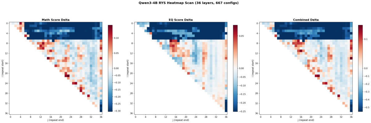
Math delta (left), EQ delta (center), and combined delta (right) across all 667 (i,j) layer duplication configs. The three-phase encode/reason/decode anatomy is clearly visible at 4B scale.
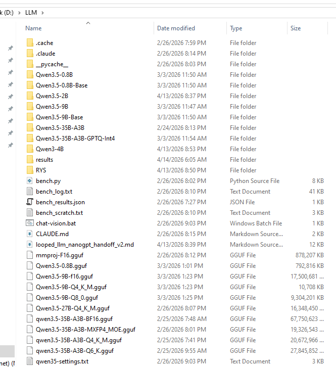
I’ve been messing around with local LLMs on my 3090 for a while now — I have a growing collection of Qwen models on D:\LLM that I probably should be embarrassed about. A few weeks ago I stumbled across David Noel Ng’s LLM Neuroanatomy blog posts, where he showed that you can take a pretrained transformer and literally just re-run some of its middle layers a second time at inference, no retraining needed, and get meaningfully better outputs.
The D:\LLM folder. I should probably be embarrassed about this.
The idea is wild: the model’s weights don’t change. You just tell it “hey, run layers 15 through 21 again” and the hidden state gets another pass through those same weights. Ng showed this working on Qwen3.5-27B (a 64-layer model) with up to +15.6% improvement on combined math and emotional reasoning benchmarks.
Naturally, I wanted to know if this works on smaller models too. Welcome to Austin’s Nerdy Things, where we perform brain surgery on 4-billion-parameter language models to make them think twice.
Background: What Is RYS?
Ng’s technique is called RYS and the core concept is surprisingly simple. A normal transformer forward pass goes:
Process input through layers 0, 1, 2, …, N-1 sequentially
Done
With RYS, you pick a contiguous block in the middle — layers i through j-1 — and after the model finishes layer j-1, you jump back and re-execute layers i through N-1. Those middle layers run twice on the evolving hidden state.
The reason this can work is that transformer layers aren’t all doing the same thing. Ng’s work showed models have a recognizable three-phase anatomy:
Early layers (~0-15% depth): Encoding. Converting tokens into contextualized representations. Repeating these produces garbage — the model tries to re-encode already-encoded stuff.
Middle layers (~20-60% depth): Reasoning. The actual thinking. Repeating these is like giving the model extra time to work through the problem.
Late layers (~70-100% depth): Decoding. Converting internal representations back into token predictions. Repeating these also produces garbage.
Ng found the sweet spot consistently in the middle, and his RYS repo provides all the tooling to test this — layer duplication wrappers, benchmark probe sets, the whole thing.
But his experiments were on a 27B model with 64 layers. I wanted to know: does this three-phase anatomy even exist at 4B scale? Can you exploit it on consumer hardware?
The Setup
Model: Qwen3-4B. I picked this one specifically because it’s a pure dense transformer (36 layers, 2560 hidden dim, GQA with 32 Q / 8 KV heads, RoPE, BF16). The Qwen3.5-2B has hybrid linear/full attention which would complicate things, and Qwen3-4B is in the same model family as Ng’s 27B target, which makes cross-scale comparison cleaner.
Hardware: My trusty RTX 3090 (24 GB VRAM). The model takes about 8.1 GB at baseline, which leaves plenty of room for the KV cache overhead from layer duplication.
Benchmarks: I used Ng’s probe sets from the RYS repo:
Math-16: 16 hard math questions (square roots, cube roots, big multiplications) requiring single-integer answers. Scored with digit-level partial credit. No chain-of-thought allowed. Greedy decoding, 64 max new tokens.
EQ-16: 16 EQ-Bench scenarios — complex social dialogues where the model predicts 4 emotion intensities on a 0-10 scale. Max 256 new tokens.
I used /no_think to disable Qwen3’s thinking mode so we’re measuring raw single-pass capability, and greedy decoding (do_sample=False), which I verified is perfectly deterministic across 5 runs on the same input. No need for multi-run variance testing.
The sweep: All 667 valid (i, j) configurations for a 36-layer model, including baseline (0, 0). Every config runs all 32 probe questions. I added early stopping that triggers if the first 2 math probes both produce garbage (saves about 30% of wall time on broken configs). The scanner saves results to JSON after every single config — resume-friendly for when Windows decides it’s update time.
Total sweep time: about 9 hours on a single 3090. Claude helped me write the scanner script (with me providing the architecture decisions and Ng’s RYS library doing the heavy lifting on layer manipulation).
Baseline Scores
Before messing with anything, Qwen3-4B scores:
Probe
Score
Math-16
0.305
EQ-16
0.749
Combined
1.054
The math score looks low, but these are genuinely hard problems (like “what is the cube root of 1019330085047 times 31?”) and the scorer gives partial credit for getting digits right. The EQ score is actually solid — Qwen3-4B is pretty decent at predicting emotional dynamics even without chain-of-thought.
The Heatmaps
Here’s where it gets fun. I swept all 667 configs and plotted the results as heatmaps. Each cell is one (i, j) configuration. Red means improvement over baseline. Blue means degradation. The x-axis is j (where the repeated block ends) and the y-axis is i (where it starts).
Left: math delta. Center: EQ delta. Right: combined delta. Red = improvement, blue = degradation. 667 configs, 36 layers.
Three things jumped out immediately.
1. The three-phase anatomy is clearly present at 4B scale
The top-left corner (early layers duplicated with wide spans) is deep blue — that’s the encoding zone. The bottom-right corner (late layers) is also blue — that’s the decoding zone. The productive region runs diagonally through the middle. This is exactly the encode / reason / decode structure Ng found at 27B.
Layers 0-6 are the encoding wall. Repeat anything starting before layer 5 with a wide span and the model outputs garbage. Layers 30+ are decoding territory — also garbage if you repeat there. The productive zone lives between layers ~5 and ~27, spanning roughly 60% of the model.
2. Math and EQ have different hot zones
This was something I wasn’t expecting. The math heatmap shows gains across a broad band from mid-stack to upper layers. The EQ heatmap’s gains concentrate in a tighter region around layers 7-16. The combined heatmap shows three distinct hot zones:
Zone A (layers 7-15, ~19-42% depth): Strong EQ gains, moderate math
Zone B (layers 15-20, ~42-56% depth): Balanced improvement on both
Zone C (layers 21-27, ~58-75% depth): Strong math gains, EQ roughly neutral
So the model’s “emotional processing” lives slightly earlier in the stack than its “mathematical processing.” That’s a cool finding — different kinds of reasoning occupy different layer ranges even in a small model.
3. The encoding wall is a cliff, not a slope
The transition from “productive duplication” to “catastrophic failure” happens over 1-2 layers. Layer 5 duplication helps. Layer 3 duplication tanks the model. There’s basically no gradient — it’s a cliff edge. Ng observed something similar at 27B but it’s even more pronounced at 4B scale.
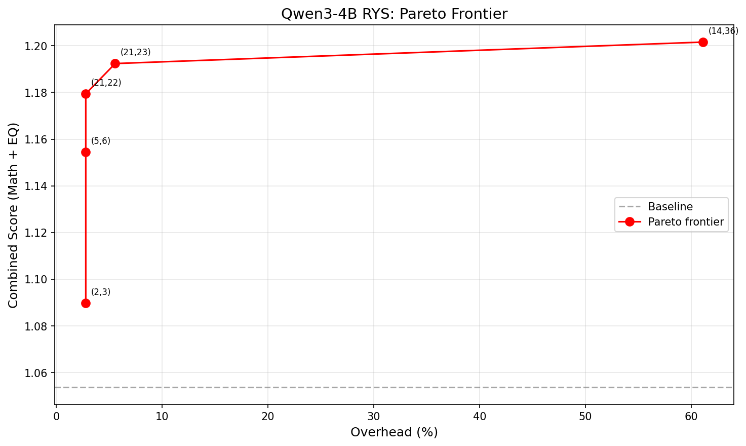
The Pareto Frontier
Not all improvements are worth the extra latency. Each extra layer traversal costs time. The practical question is: how much bang per buck?
X-axis: overhead (%). Y-axis: combined score. The curve is sharply concave — almost all the benefit comes from the first 1-2 extra layers.
Size
Config (i,j)
Extra layers
Overhead
Combined
Improvement
XS
(2,3)
1
2.8%
1.090
+3.4%
S
(5,6)
1
2.8%
1.154
+9.6%
M
(21,22)
1
2.8%
1.179
+11.9%
L
(21,23)
2
5.6%
1.192
+13.2%
XL
(14,36)
22
61.1%
1.202
+14.0%
The winner is (21,22): just repeat layer 21 once. That’s +11.9% combined improvement at 2.8% latency overhead. One single extra layer forward pass. That’s it.
Going from 1 extra layer to 2 buys another 1.3 percentage points. Going from 2 extra layers to 22 — literally 10x the overhead — buys only 0.8 more. The returns collapse fast. Look at that Pareto chart — the curve is basically flat after the first couple of points.
Single-Layer Repeats: The 4B Surprise
This is where things get really interesting, and where the results diverge most from Ng’s 27B findings.
Ng reported that single-layer repeats at 27B “almost never help.” You need to duplicate a contiguous block of at least 2-3 layers to see meaningful improvement at that scale.
At 4B? 14 out of 35 single-layer repeats beat baseline. Here are the top performers:
Layer
Config
Combined delta
21
(21,22)
+0.126
5
(5,6)
+0.101
24
(24,25)
+0.100
26
(26,27)
+0.073
19
(19,20)
+0.071
22
(22,23)
+0.063
20
(20,21)
+0.057
17
(17,18)
+0.049
Layers 5 and 17-26 — nearly the entire mid-to-late stack — all produce meaningful gains when repeated individually. That’s a wide, diffuse productive zone spanning about 60% of the model.
My interpretation: smaller models have less specialized layers. At 27B with 64 layers, each layer does something specific enough that repeating just one doesn’t help much — you need a coherent block. At 4B with 36 layers, individual layers carry more general-purpose reasoning capacity. A single extra pass through one of them is already enough to bump quality.
This is arguably the most practically useful finding from the whole experiment. For small models, even the simplest possible intervention works.
How This Compares to Ng’s 27B Results
Property
Qwen3-4B (36 layers)
Qwen3.5-27B (64 layers)
Three-phase anatomy
Yes, clearly visible
Yes
Encoding wall
Layers 0-6 (~0-17%)
~first 15%
Best single-layer
(21,22) = +11.9%
Rarely productive
Best absolute
(14,36) = +14.0% at 61% overhead
~+15.6% at ~15.6% overhead
Best efficiency
(21,22) = +11.9% at 2.8% overhead
Layer 33 = +1.5%
Productive single layers
14/35 (40%)
Rare
Efficiency curve shape
Sharply concave
Roughly linear to ~10 layers
The biggest difference is the shape of the efficiency curve. At 27B, adding more repeated layers gives roughly linear improvement up to about 10 extra layers — there’s a real reason to invest in multi-layer duplication. At 4B, the curve is sharply concave. Almost all the benefit comes from the very first extra layer. After that, you’re paying a lot of overhead for very little gain.
This makes intuitive sense. A bigger model has more specialized layers where repetition compounds — each one contributes something distinct. A smaller model gets most of its benefit from a single extra pass through its most general-purpose reasoning layer, and additional passes hit diminishing returns because those layers are doing similar work.
What This Means If You Want to Use It
If you’re deploying a small dense model and want better reasoning at minimal cost:
Find the model’s “layer 21.” Run a quick single-layer sweep on your target model. It takes minutes per config.
Repeat that one layer. At 2.8% latency overhead, this is basically free.
Don’t over-invest in multi-layer duplication at small scale. The second extra layer buys way less than the first.
For framework implementers: this is a ~10-line change to a model’s forward pass. No weight changes, no retraining, no meaningful VRAM increase. It should be a first-class inference option in llama.cpp, vLLM, ExLlama, etc.
Caveats
I want to be upfront about what this doesn’t prove:
One model, one family. These results are Qwen3-4B specific. The three-phase anatomy probably generalizes (Ng showed it on multiple architectures), but the exact layer numbers won’t. Every model needs its own sweep.
Small probe sets. 16 math + 16 EQ questions. Enough for relative ordering of configs, but the absolute scores have meaningful variance. Validate on larger benchmarks before deploying.
Greedy decoding only. Sampling might interact differently with layer duplication. I haven’t tested that.
No multi-block compositions. Ng’s beam search finds configs that repeat two different blocks (e.g., layers 30-34 AND 43-45). I only tested single contiguous blocks. The multi-block space at 4B is unexplored.
RoPE positions aren’t adjusted. The model sees the same position IDs on the repeated pass. This works empirically but the theoretical interaction is unclear.
Reproducing This
Everything runs on a single 3090 (or any 24GB+ GPU):
The scanner loads the model once, pre-tokenizes all probes, then iterates through configs. Each config wraps the base model with a layer-index remapping (no weight copies, just pointer rearrangement), runs all probes greedy, scores, and saves. Resume works by checking which config keys already exist in the results JSON.
What’s Next
A few obvious follow-ups I’m thinking about:
Multi-block beam search at 4B. Does combining layers 5-6 and 21-22 compound the gains?
Cross-scale comparison. Run the same sweep on Qwen3.5-2B (hybrid attention), Qwen3.5-9B, maybe a non-Qwen model. See how the efficiency curve changes with scale.
Train-time loop exposure. Train a small model where specific layers are looped during training, compare with inference-time-only duplication.
Integration with inference frameworks. llama.cpp, vLLM, and ExLlama already manage layer weights — adding a “repeat layer N” flag should be pretty straightforward.
The broader takeaway is that transformer layers aren’t interchangeable. They have structure, and that structure is legible even at small scale. You can exploit it at inference time with zero retraining, and the cost is basically nothing.
Layer 21 thinks twice. The model gets smarter. That’s the whole trick.
I’ve been building SkySpottr, an AR app overlaying aircraft information on your phone’s screen, using your device’s location, orientation, and incoming aircraft data (ADS-B) to predict where planes should appear on screen, then uses a YOLO model to lock onto the actual aircraft and refine the overlay. YOLOv8 worked great for this… until I actually read the license.
Welcome to Austin’s Nerdy Things, where we train from scratch entire neural networks to avoid talking to lawyers.
The Problem with Ultralytics
YOLOvWhatver is excellent. Fast, accurate, easy to use, great documentation. But Ultralytics licenses it under AGPL-3.0, which means if you use it in a product, you either need to open-source your entire application or pay for a commercial license. For a side project AR app that I might eventually monetize? That’s a hard pass.
Enter YOLOX from Megvii (recommended by either ChatGPT or Claude, can’t remember which, as an alternative). MIT licensed. Do whatever you want with it. The catch? You have to train your own models from scratch instead of using Ultralytics’ pretrained weights and easy fine-tuning pipeline. I have since learned there are some pretrained models. I didn’t use them.
So training from scratch is what I did. Over a few late nights in December 2025, I went from zero YOLOX experience to running custom-trained aircraft detection models in my iOS app. Here’s how it went.
The Setup
Hardware: RTX 3090 on my Windows machine, COCO2017 dataset on network storage (which turned out to be totally fine for training speed), and way too many terminal windows open.
I started with the official YOLOX repo and the aircraft class from COCO2017. The dataset has about 3,000 training images with airplanes, which is modest but enough to get started.
The first training run failed immediately because I forgot to install YOLOX as a package. Classic. Then it failed again because I was importing a class that didn’t exist in the version I had. Claude (who was helping me through this, and hallucinated said class) apologized and fixed the import. We got there eventually.
Training Configs: Nano, Tiny, Small, and “Nanoish”
YOLOX has a nice inheritance-based config system. You create a Python file, inherit from a base experiment class, and override what you want. I ended up with four different configs:
yolox_nano_aircraft.py – The smallest. 0.9M params, 1.6 GFLOPs. Runs on anything.
yolox_tiny_aircraft.py – Slightly bigger with larger input size for small object detection.
yolox_small_aircraft.py – 5M params, 26 GFLOPs. The “serious” model.
yolox_nanoish_aircraft.py – My attempt at something between nano and tiny.
The “nanoish” config was my own creation where I tried to find a sweet spot. I bumped the width multiplier from 0.25 to 0.33 and… immediately got a channel mismatch error because 0.33 doesn’t divide evenly into the architecture. Turns out you can’t just pick arbitrary numbers. I am a noob at these things. Lesson learned.
After some back-and-forth, I settled on a config with 0.3125 width (which is 0.25 \* 1.25, mathematically clean) and 512×512 input. This gave me roughly 1.2M params – bigger than nano, smaller than tiny, and it actually worked.
Here’s the small model config – the one that ended up in production. The key decisions are width = 0.50 (2x wider than nano for better feature extraction), 640×640 input for small object detection, and full mosaic + mixup augmentation:
class Exp(MyExp):
    def __init__(self):
        super(Exp, self).__init__()

        # Model config - YOLOX-Small architecture
        self.num_classes = 1  # Single class: airplane
        self.depth = 0.33
        self.width = 0.50  # 2x wider than nano for better feature extraction

        # Input/output config - larger input helps small object detection
        self.input_size = (640, 640)
        self.test_size = (640, 640)
        self.multiscale_range = 5  # Training will vary from 480-800

        # Data augmentation
        self.mosaic_prob = 1.0
        self.mosaic_scale = (0.1, 2.0)
        self.enable_mixup = True
        self.mixup_prob = 1.0
        self.flip_prob = 0.5
        self.hsv_prob = 1.0

        # Training config
        self.warmup_epochs = 5
        self.max_epoch = 400
        self.no_aug_epochs = 100
        self.basic_lr_per_img = 0.01 / 64.0
        self.scheduler = "yoloxwarmcos"

    def get_model(self):
        from yolox.models import YOLOX, YOLOPAFPN, YOLOXHead

        in_channels = [256, 512, 1024]
        # Small uses standard convolutions (no depthwise)
        backbone = YOLOPAFPN(self.depth, self.width, in_channels=in_channels, act=self.act)
        head = YOLOXHead(self.num_classes, self.width, in_channels=in_channels, act=self.act)
        self.model = YOLOX(backbone, head)
        return self.model
And the nanoish config for comparison – note the depthwise=True and the width of 0.3125 (5/16) that I landed on after the channel mismatch debacle:
class Exp(MyExp):
    def __init__(self):
        super(Exp, self).__init__()

        self.num_classes = 1
        self.depth = 0.33
        self.width = 0.3125  # 5/16 - halfway between nano (0.25) and tiny (0.375)

        self.input_size = (512, 512)
        self.test_size = (512, 512)

        # Lighter augmentation than small - this model is meant to be fast
        self.mosaic_prob = 0.5
        self.mosaic_scale = (0.5, 1.5)
        self.enable_mixup = False

    def get_model(self):
        from yolox.models import YOLOX, YOLOPAFPN, YOLOXHead

        in_channels = [256, 512, 1024]
        backbone = YOLOPAFPN(self.depth, self.width, in_channels=in_channels,
                             act=self.act, depthwise=True)  # Depthwise = lighter
        head = YOLOXHead(self.num_classes, self.width, in_channels=in_channels,
                         act=self.act, depthwise=True)
        self.model = YOLOX(backbone, head)
        return self.model
The -c yolox_s.pth loads YOLOX’s pretrained COCO weights as a starting point (transfer learning). The -d 1 is one GPU, -b 16 is batch size 16 (about 8GB VRAM on the 3090 with fp16), and --fp16 enables mixed precision training.
The Small Object Problem
Here’s the thing about aircraft detection for an AR app: planes at cruise altitude look tiny. A 747-8 at 37,000 feet is maybe 20-30 pixels on your phone screen if you’re lucky, even with the 4x optical zoom of the newest iPhones (8x for the 12MP weird zoom mode). Standard YOLO models are tuned for reasonable-sized objects, not specks in the sky. The COCO dataset has aircraft that are reasonably sized, like when you’re sitting at your gate at an airport and take a picture of the aircraft 100 ft in front of you.
My first results were underwhelming. The nano model was detecting larger aircraft okay but completely missing anything at altitude. The evaluation metrics looked like this:
AP for airplane = 0.234
AR for small objects = 0.089
Not great. The model was basically only catching aircraft on approach or takeoff.
For the small config, I made some changes to help with tiny objects:
Increased input resolution to 640×640 (more pixels = more detail for small objects)
Enabled full mosaic and mixup augmentation (helps the model see varied object scales)
Switched from depthwise to regular convolutions (more capacity)
(I’ll be honest, I was leaning heavily on Claude for the ML-specific tuning decisions here)
This pushed the model to 26 GFLOPs though, which had me worried about phone performance.
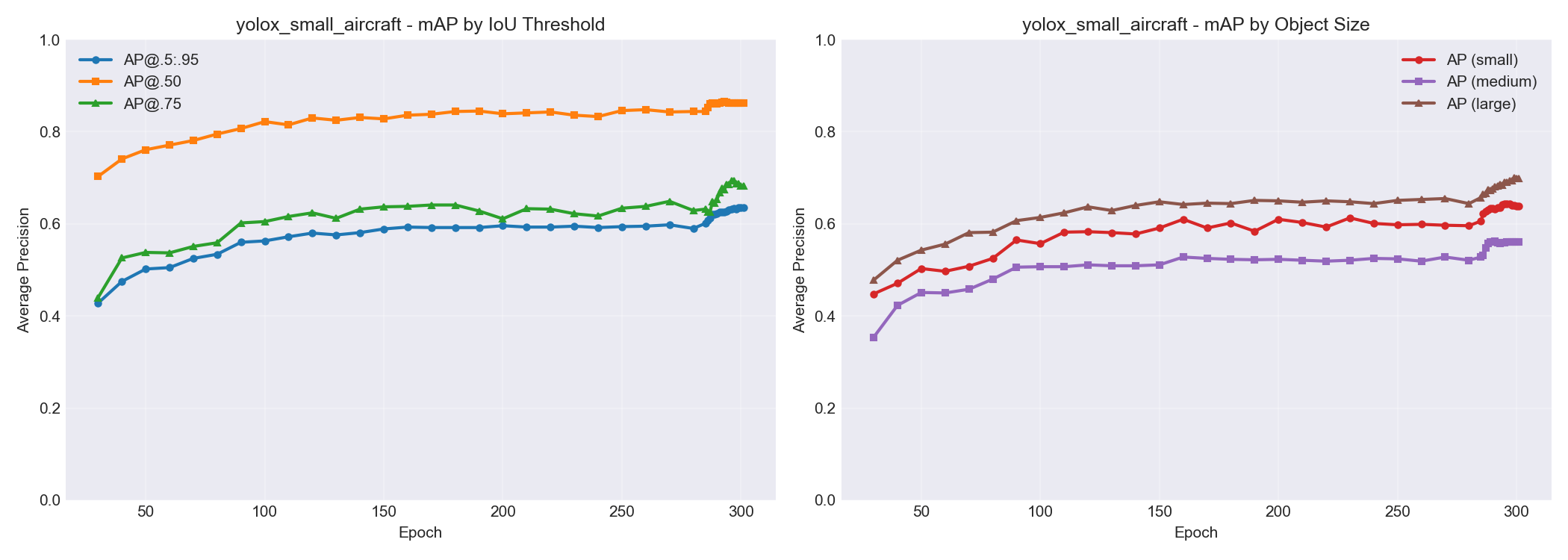
Here’s what the small model’s accuracy looked like broken down by object size. You can see AP for small objects climbing from ~0.45 to ~0.65 over training, while large objects hit ~0.70. Progress, but small objects remain the hardest category – which tracks with the whole “specks in the sky” problem.
Will This Actually Run on a Phone?
The whole point of this exercise was to run inference on an iPhone. So here is some napkin math:
Model
GFLOPs
Estimated Phone Inference
Nano
1.6
~15ms, smooth 30fps easy
Nanoish
3.2
~25ms, still good
Small
26
~80ms, might be sluggish
YOLOv8n (for reference)
8.7
~27ms
My app was already running YOLOv8n at 15fps with plenty of headroom. So theoretically even the small model should work, but nano/nanoish would leave more room for everything else the app needs to do.
The plan: train everything, compare accuracy, quantize for deployment, and see what actually works in practice.
Training Results (And a Rookie Mistake)
After letting things run overnight (300 epochs takes a while even on a 3090), here’s what I got:
The nanoish model at epoch 100 was already showing 94% detection rate on test images, beating the fully-trained nano model. And it wasn’t even done training yet.
Quick benchmark on 50 COCO test images with aircraft (RTX 3090 GPU inference – not identical to phone, but close enough for the smaller models to be representative):
Model
Detection Rate
Avg Detections/Image
Avg Inference (ms)
FPS
YOLOv8n
58.6%
0.82
33.6
29.7
YOLOX nano
74.3%
1.04
14.0
71.4
YOLOX nanoish
81.4%
1.14
15.0
66.9
YOLOX tiny
91.4%
1.28
16.5
60.7
YOLOX small
92.9%
1.30
17.4
57.4
Ground Truth
–
1.40
–
–
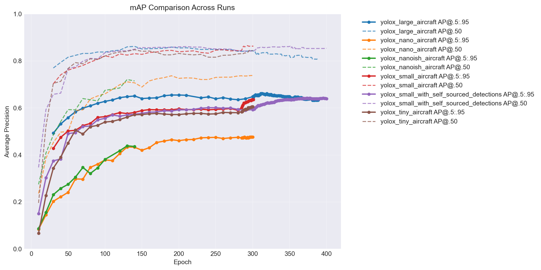
YOLOv8n getting beaten by every single YOLOX variant while also being slower was… not what I expected. Here’s the mAP comparison across all the models over training – you can see the hierarchy pretty clearly:
The big takeaway: more capacity = better accuracy, but with diminishing returns. The jump from nano to nanoish is huge, nanoish to small is solid, and tiny lands somewhere in between depending on the epoch. (You’ll notice two extra lines in the chart – a large model and a self-sourced variant. I kept training after this post’s story ends. More on the self-sourced pipeline later. You can also see the large model is clearly overfitting past epoch ~315 – loss keeps decreasing but mAP starts dropping. My first time overfitting a model.)
The nanoish model hit a nice sweet spot. Faster than YOLOv8n, better small object detection than pure nano, and still lightweight enough for mobile.
And here is the output from my plot_training.py script:
But there was a problem I didn’t notice until later: my training dataset had zero images without aircraft in them. Every single training image contained at least one airplane. This is… not ideal if you want your model to learn what an airplane isn’t. More on that shortly.
How It Actually Works in the App
Before I get to results, here’s what the ML is actually doing in SkySpottr. The app combines multiple data sources to track aircraft:
ADS-B data tells us where aircraft are in 3D space (lat, lon, altitude)
Device GPS and orientation tell us where the phone is and which way it’s pointing
Physics-based prediction places aircraft overlays on screen based on all the above
That prediction is usually pretty good, but phone sensors drift and aircraft positions are slightly delayed. So the overlays can be off by a couple degrees. This is where YOLO comes in.
The app runs the model on each camera frame looking for aircraft. When it finds one within a threshold distance of where the physics engine predicted an aircraft should be, it “snaps” the overlay to the actual detected position. The UI shows an orange circle around the aircraft and marks it as “SkySpottd” – confirmed via machine learning.
I call this “ML snap” mode. It’s the difference between “there’s probably a plane somewhere around here” and “that specific bright dot is definitely the aircraft.”
The model runs continuously on device, which is why inference time matters so much. Even at 15fps cap, that’s still 15 inference cycles per second competing with everything else the app needs to do (sensor fusion, WebSocket data, AR rendering, etc.). Early on I was seeing 130%+ CPU usage on my iPhone, which is not great for battery life. Every millisecond saved on inference is a win.
Getting YOLOX into CoreML
One thing the internet doesn’t tell you: YOLOX and Apple’s Vision framework don’t play nice together.
YOLOv8 exports to CoreML with a nice Vision-compatible interface. You hand it an image, it gives you detections. Easy. YOLOX expects different preprocessing – it wants pixel values in the 0-255 range (not normalized 0-1), and the output tensor layout is different.
The conversion pipeline goes PyTorch → TorchScript → CoreML. Here’s the core of it:
import torch
import coremltools as ct
from yolox.models import YOLOX, YOLOPAFPN, YOLOXHead

# Build model (same architecture as training config)
backbone = YOLOPAFPN(depth=0.33, width=0.50, in_channels=[256, 512, 1024], act="silu")
head = YOLOXHead(num_classes=1, width=0.50, in_channels=[256, 512, 1024], act="silu")
model = YOLOX(backbone, head)

# Load trained weights
ckpt = torch.load("yolox_small_best.pth", map_location="cpu", weights_only=False)
model.load_state_dict(ckpt["model"])
model.eval()
model.head.decode_in_inference = True  # Output pixel coords, not raw logits

# Trace and convert
dummy = torch.randn(1, 3, 640, 640)
traced = torch.jit.trace(model, dummy)
mlmodel = ct.convert(
    traced,
    inputs=[ct.TensorType(name="images", shape=(1, 3, 640, 640))],
    outputs=[ct.TensorType(name="output")],
    minimum_deployment_target=ct.target.iOS15,
    convert_to="mlprogram",
)
mlmodel.save("yolox_small_aircraft.mlpackage")
The decode_in_inference = True is crucial — without it, the model outputs raw logits and you’d need to implement the decode head in Swift. With it, the output is [1, N, 6] where 6 is [x_center, y_center, width, height, obj_conf, class_score] in pixel coordinates.
On the Swift side, Claude ended up writing a custom detector that bypasses the Vision framework entirely. Here’s the preprocessing — the part that was hardest to get right:
/// Convert pixel buffer to MLMultiArray [1, 3, H, W] with 0-255 range
private func preprocess(pixelBuffer: CVPixelBuffer) -> MLMultiArray? {
    // GPU-accelerated resize via Core Image
    let ciImage = CIImage(cvPixelBuffer: pixelBuffer)
    let scaleX = CGFloat(inputSize) / ciImage.extent.width
    let scaleY = CGFloat(inputSize) / ciImage.extent.height
    let scaledImage = ciImage.transformed(by: CGAffineTransform(scaleX: scaleX, y: scaleY))

    // Reuse pixel buffer from pool (memory leak fix #1)
    var resizedBuffer: CVPixelBuffer?
    CVPixelBufferPoolCreatePixelBuffer(kCFAllocatorDefault, pool, &resizedBuffer)
    guard let buffer = resizedBuffer else { return nil }
    ciContext.render(scaledImage, to: buffer)

    // Reuse pre-allocated MLMultiArray (memory leak fix #2)
    guard let array = inputArray else { return nil }

    CVPixelBufferLockBaseAddress(buffer, .readOnly)
    defer { CVPixelBufferUnlockBaseAddress(buffer, .readOnly) }

    let bytesPerRow = CVPixelBufferGetBytesPerRow(buffer)
    let pixels = CVPixelBufferGetBaseAddress(buffer)!.assumingMemoryBound(to: UInt8.self)
    let arrayPtr = array.dataPointer.assumingMemoryBound(to: Float.self)
    let channelStride = inputSize * inputSize

    // BGRA → RGB, keep 0-255 range (YOLOX expects unnormalized pixels)
    // Direct pointer access is ~100x faster than MLMultiArray subscript
    for y in 0..<inputSize {
        let rowOffset = y * bytesPerRow
        let yOffset = y * inputSize
        for x in 0..<inputSize {
            let px = rowOffset + x * 4
            let idx = yOffset + x
            arrayPtr[idx] = Float(pixels[px + 2])                      // R
            arrayPtr[channelStride + idx] = Float(pixels[px + 1])      // G
            arrayPtr[2 * channelStride + idx] = Float(pixels[px])      // B
        }
    }
    return array
}
The two key gotchas: (1) BGRA byte order from the camera vs RGB that the model expects, and (2) YOLOX wants raw 0-255 pixel values, not the 0-1 normalized range that most CoreML models expect. If you normalize, everything silently breaks — the model runs, returns garbage, and you spend an evening wondering why.
For deployment, I used CoreML’s INT8 quantization (coremltools.optimize.coreml.linear_quantize_weights). This shrinks the model by about 50% with minimal accuracy loss. The small model went from ~17MB to 8.7MB, and inference time improved slightly.
Real World Results (Round 1)
I exported the nanoish model and got it running in SkySpottr. The good news: it works. The ML snap feature locks onto aircraft, the orange verification circles appear, and inference is fast enough that I don’t notice any lag.
The less good news: false positives. Trees, parts of houses, certain cloud formations – the model occasionally thinks these are aircraft. Remember that rookie mistake about no negative samples? Yeah.
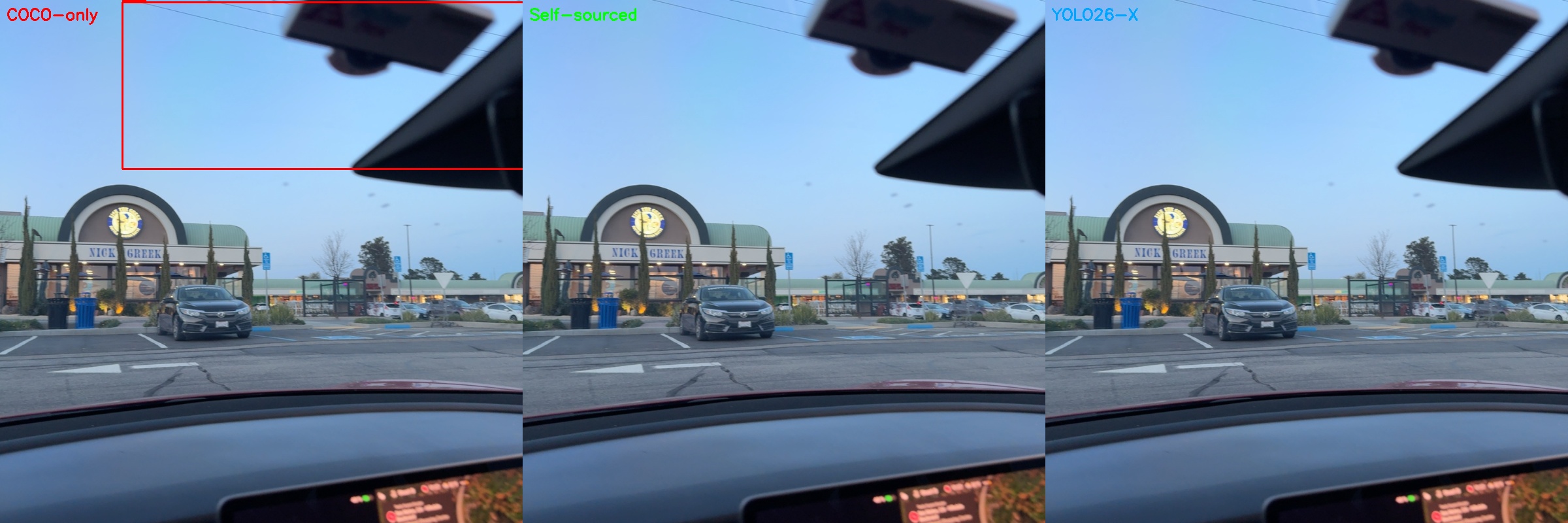
I later set up a 3-way comparison to visualize exactly this kind of failure. The three panels show my COCO-only trained model (red boxes), a later model trained on self-sourced images (green boxes – I’ll explain this pipeline shortly), and YOLO26-X as a ground truth oracle (right panel, no boxes means no detection). The COCO-only model confidently detects an “aircraft” that is… a building. The other two correctly ignore it.
The app handles this gracefully because of the matching threshold. Random false positives in empty sky don’t trigger the snap because there’s no predicted aircraft nearby to match against. But when there’s a tree branch right next to where a plane should be, the model sometimes locks onto the wrong thing.
The even less good news: it still struggles with truly distant aircraft. A plane at 35,000 feet that’s 50+ miles away is basically a single bright pixel. No amount of ML is going to reliably detect that. For those, the app falls back on pure ADS-B prediction, which is usually good enough to get the overlay in the right general area.
But when it works, it works. I’ll show some examples of successful detections in the self-sourced section below.
The Memory Leak Discovery (Fun Debugging Tangent)
While testing the YOLOX integration, I was also trying to get RevenueCat working for subscriptions. Had the app running for about 20 minutes while I debugged the in-app purchase flow. Noticed it was getting sluggish, opened Instruments, and… yikes.
Base memory for the app is around 200MB. After 20 minutes of continuous use, it had climbed to 450MB. Classic memory leak pattern.
The culprit was AI induced, and AI resolved: it was creating a new CVPixelBuffer and MLMultiArray for every single frame. At 15fps, that’s 900 allocations per minute that weren’t getting cleaned up fast enough.
The fix was straightforward – use a CVPixelBufferPool for the resize buffers and pre-allocate a single MLMultiArray that gets reused. Memory now stays flat even after hours of use.
(The RevenueCat thing? I ended up ditching it entirely and going with native StoreKit2. RevenueCat is great, but keeping debug and release builds separate was more hassle than it was worth for a side project. StoreKit2 is actually pretty nice these days if you don’t need the analytics. I’m at ~80 downloads, and not a single purchase. First paid app still needs some fine tuning, clearly, on the whole freemium thing.)
Round 2: Retraining with Negative Samples
After discovering the false positive issue, I went back and retrained. This time I made sure to include images without aircraft – random sky photos, clouds, trees, buildings, just random COCO2017 stuff. The model needs to learn what’s NOT an airplane just as much as what IS one.
Here’s the extraction script that handles the negative sampling. The key insight: you need to explicitly tell the model what empty sky looks like:
def extract_airplane_dataset(split="train", negative_ratio=0.2, seed=42):
    """Extract airplane images from COCO, with negative samples."""
    with open(f"instances_{split}2017.json") as f:
        coco_data = json.load(f)

    # Find all images WITH airplanes
    airplane_image_ids = set()
    for ann in coco_data['annotations']:
        if ann['category_id'] == AIRPLANE_CATEGORY_ID:  # 5 in COCO
            airplane_image_ids.add(ann['image_id'])

    # Find images WITHOUT airplanes for negative sampling
    all_ids = {img['id'] for img in coco_data['images']}
    negative_ids = all_ids - airplane_image_ids

    # Add 20% negative images (no airplanes = teach model what ISN'T a plane)
    num_negatives = int(len(airplane_image_ids) * negative_ratio)
    sampled_negatives = random.sample(list(negative_ids), num_negatives)
    # ... copy images and annotations to output directory
I also switched from nanoish to the small model. The accuracy improvement on distant aircraft was worth the extra compute, and with INT8 quantization the inference time came in at around 5.6ms on an iPhone – way better than my napkin math predicted. Apple’s Neural Engine is impressive.
The final production model: YOLOX-Small, 640×640 input, INT8 quantized, ~8.7MB on disk. It runs at 15fps with plenty of headroom for the rest of the app on my iPhone 17 Pro.
Round 3: Self-Sourced Images and Closing the Loop
So the model works, but it was trained entirely on COCO2017 – airport tarmac photos, stock images, that kind of thing. My app is pointing at the sky from the ground. Those are very different domains.
I added a debug flag to SkySpottr for my phone that saves every camera frame where the model fires a detection. Just flip it on, walk around outside for a while, and the app quietly collects real-world training data. Over a few weeks of casual use, I accumulated about 2,000 images from my phone.
The problem: these images don’t have ground truth labels. I’m not going to sit there and manually draw bounding boxes on 2,000 sky photos. So I used YOLO26-X (Ultralytics’ latest and greatest, which I’m fine using as an offline tool since it never ships in the app) as a teacher model. Run it on all the collected images, take its high-confidence detections as pseudo-labels, convert to COCO annotation format, and now I have a self-sourced dataset to mix in with the original COCO training data.
Here’s the pseudo-labeling pipeline. First, run the teacher model on all collected images:
from ultralytics import YOLO

model = YOLO("yolo26x.pt")  # Big model, accuracy over speed

for img_path in tqdm(image_paths, desc="Processing images"):
    results = model(str(img_path), conf=0.5, verbose=False)
    boxes = results[0].boxes
    airplane_boxes = boxes[boxes.cls == AIRPLANE_CLASS_ID]

    for box in airplane_boxes:
        xyxy = box.xyxy[0].cpu().numpy().tolist()
        x1, y1, x2, y2 = xyxy
        detections.append({
            "bbox_xywh": [x1, y1, x2 - x1, y2 - y1],  # COCO format
            "confidence": float(box.conf[0]),
        })
Then convert those detections to COCO annotation format so YOLOX can train on them:
def convert_to_coco(detections):
    """Convert YOLO26 detections to COCO training format."""
    coco_data = {
        "images": [], "annotations": [],
        "categories": [{"id": 1, "name": "airplane", "supercategory": "vehicle"}],
    }

    for uuid, data in detections.items():
        img_path = Path(data["image_path"])
        width, height = Image.open(img_path).size

        if width > 1024 or height > 1024:  # Skip oversized images
            continue

        coco_data["images"].append({"id": image_id, "file_name": f"{uuid}.jpg",
                                     "width": width, "height": height})

        for det in data["detections"]:
            coco_data["annotations"].append({
                "id": ann_id, "image_id": image_id, "category_id": 1,
                "bbox": det["bbox_xywh"], "area": det["bbox_xywh"][2] * det["bbox_xywh"][3],
                "iscrowd": 0,
            })

    with open("instances_train.json", "w") as f:
        json.dump(coco_data, f)
Finally, combine both datasets in the training config using YOLOX’s ConcatDataset:
Out of 2,000 images, YOLO26-X found aircraft in about 108 of them at a 0.5 confidence threshold – a 1.8% hit rate, which makes sense since most frames are just empty sky between detections. I filtered out anything over 1024px and ended up with a nice supplementary dataset of aircraft-from-the-ground images.
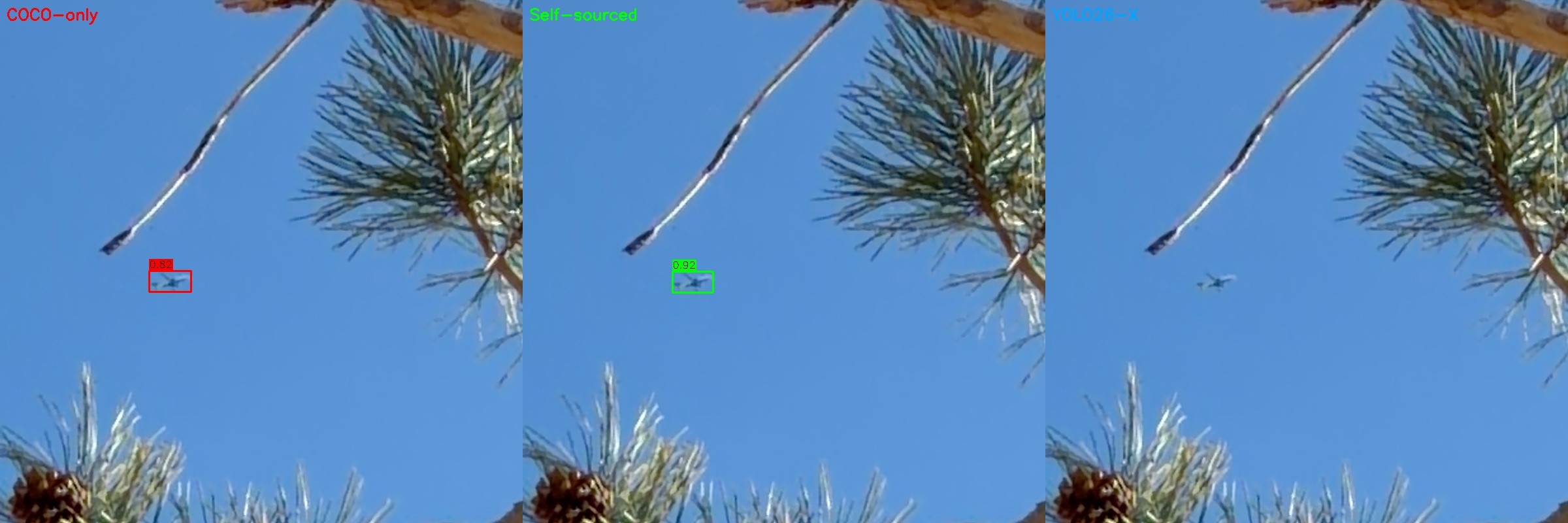
The 3-way comparison images I showed earlier came from this pipeline. Here’s what successful detections look like – the COCO-only model (red), self-sourced model (green), and YOLO26-X (right panel, shown at full resolution so you can see what we’re actually detecting):
That’s maybe 30 pixels of airplane against blue sky, detected with 0.88 and 0.92 confidence by the two YOLOX variants.
And here’s one I particularly like – aircraft spotted through pine tree branches. Real-world conditions, not a clean test image. Both YOLOX models nail it, YOLO26-X misses at this confidence threshold:
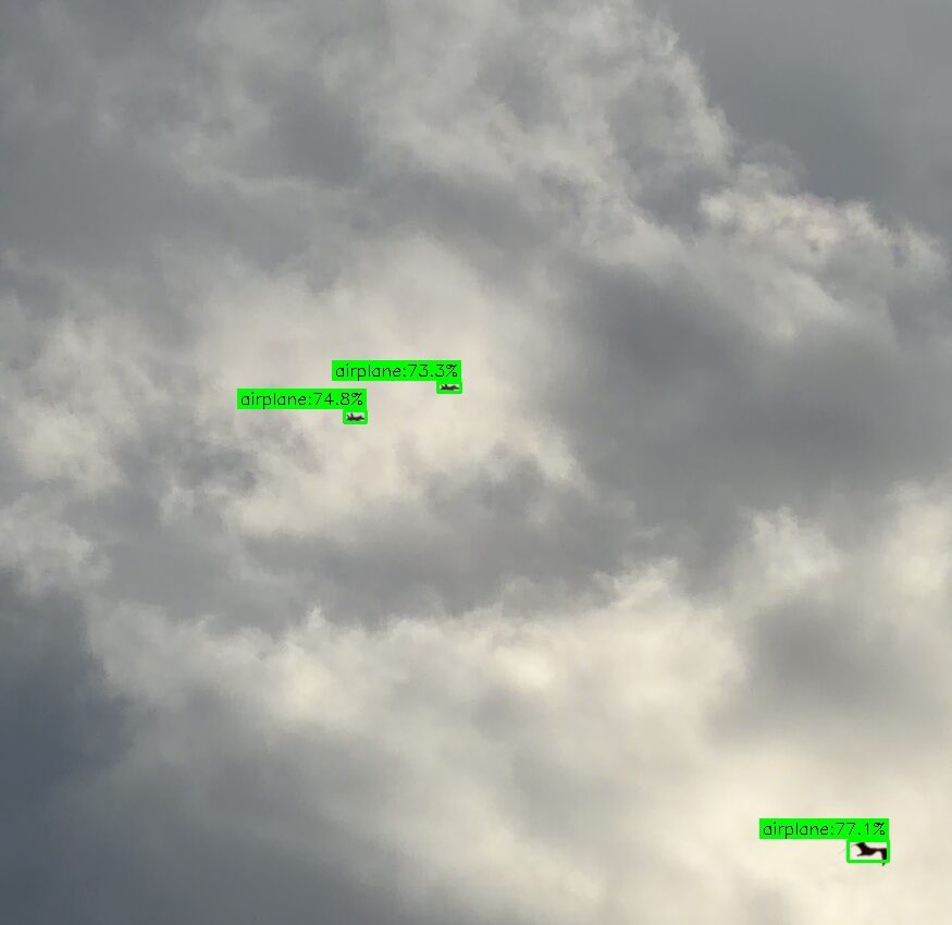
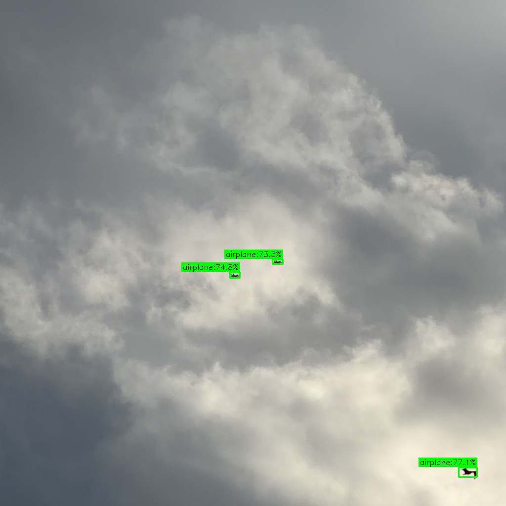
And a recent one from February 12, 2026 – a pair of what appear to be F/A-18s over Denver at 4:22 PM MST, captured at 12x zoom. The model picks up both jets at 73-75% confidence, plus the bird in the bottom-right at 77% (a false positive the app filters out via ADS-B matching). Not bad for specks against an overcast sky.
I also trained a full YOLOX-Large model (depth 1.0, width 1.0, 1024×1024 input) on the combined dataset, just to see how far I could push it. Too heavy for phone deployment, but useful for understanding the accuracy ceiling.
Conclusion
Was this worth it to avoid Ultralytics’ licensing? Since it took an afternoon and a couple evenings of vibe-coding, yes, it was not hard to switch. Not just because MIT is cleaner than AGPL, but because I learned a ton about how these models actually work. The Ultralytics ecosystem is so polished that it’s easy to treat it as a black box. Building from YOLOX forced me to understand some of the nuances, the training configs, and the tradeoffs between model size and accuracy.
Plus, I can now say I trained my own object detection model from scratch. That’s worth something at parties. Nerdy parties, anyway.
SkySpottr is live on the App Store if you want to see the model in action – point your phone at the sky and watch it lock onto aircraft in real-time.
The self-sourced pipeline is still running. Every time I use the app with the debug flag on, it collects more training data. The plan is to periodically retrain as the dataset grows – especially now that I’m getting images from different weather conditions, times of day, and altitudes. The COCO-only model was a solid start, but a model trained on actual ground-looking-up images of aircraft at altitude? That’s the endgame.
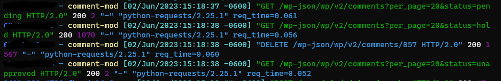
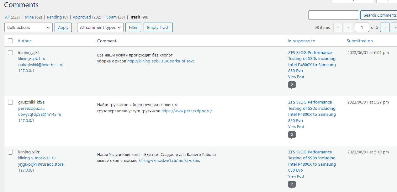
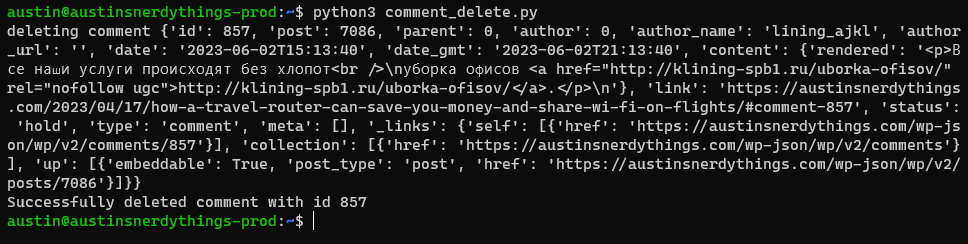
Like all other WordPress blogs, this one attracts a good number of spam comments. I get usually 5-10 per day, but yesterday there were like 30. Almost all of them contain Cyrillic characters:
Since I specify that all comments are held until approved, that means I need to either approve or trash or spam every comment.
Enter ChatGPT
I use ChatGPT (specifically GPT 4) for a number of minor coding tasks. I find it helpful. It is not perfect. That doesn’t mean it isn’t useful. I decided to have it ponder this issue. I work with Python a lot at work and it’s typically my scripting language of choice. My initial request is as follows:
write a python script to log into a wordpress site as an admin, get the top 5 comments, see if there are any Cyrillic characters in them, and if there are, delete said comment
It was understandably unhappy about potentially being asked to “hack” a WordPress site, so I had to reassure it that I was the owner of said site:
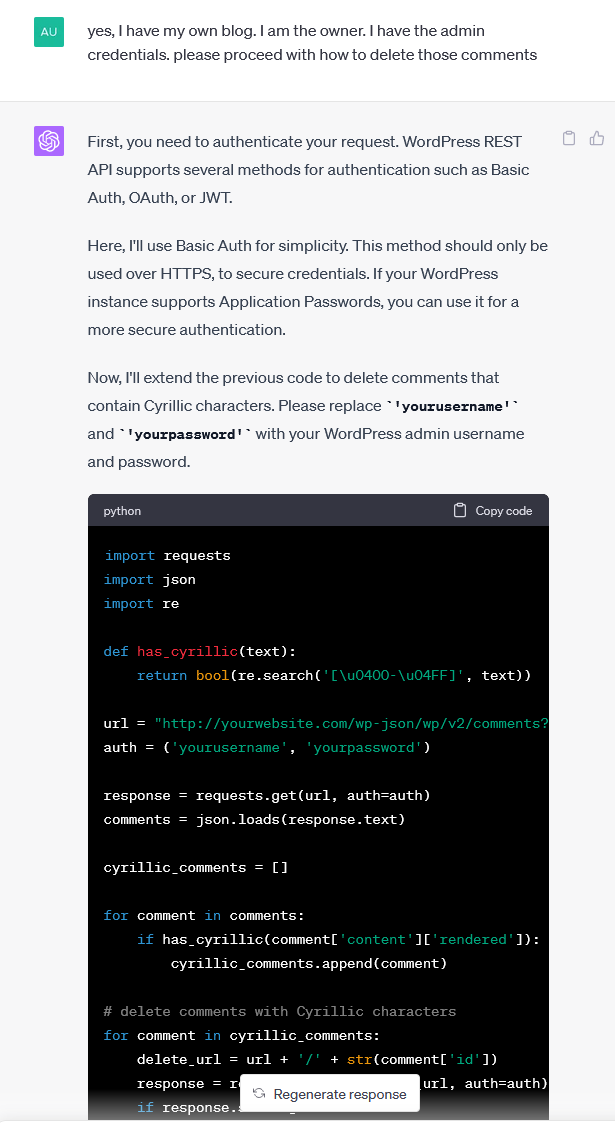
yes, I have my own blog. I am the owner. I have the admin credentials. please proceed with how to delete those comments
It happily complied and spit out some very usable code:
After a bit more back and forth:
does this get comments in a pending state? I don't let them be published instantly because most of them are spam
I was informed there are 5 different comment states: approved, hold, spam, trash, unapproved.
perfect. can you please adjust the script to get the pending, unapproved, and hold comments. also make it top 20
It ran perfectly after copy + pasting the Python. Unfortunately I created an application password for my main login on this site and forgot to change the delete URL so it happily sent my application password and username to yourwebsite.com. After revoking that password and realizing there should be a base url:
please split out the site url (https://austinsnerdythings.com) from base_url for both retrieving the comments as well as deleting
I was left with a 100% functional script. This took 3-4 min of back and forth with ChatGPT 4.0. I definitely could’ve code this up myself with the basic structure in 15 minutes or so but I would’ve had to work out the json format for comments and all that. It is so much easier to just test out what ChatGPT provides and alter as necessary:
import requests
import json
import re

def has_cyrillic(text):
    return bool(re.search('[\u0400-\u04FF]', text))

site_url = "https://austinsnerdythings.com"
base_url = f"{site_url}/wp-json/wp/v2/comments?per_page=20&status="
statuses = ['pending', 'hold', 'unapproved']
auth = ('yourusername', 'yourpassword')

for status in statuses:
    url = base_url + status
    response = requests.get(url, auth=auth)
    comments = json.loads(response.text)

    cyrillic_comments = []

    for comment in comments:
        if has_cyrillic(comment['content']['rendered']):
            cyrillic_comments.append(comment)

    # delete comments with Cyrillic characters
    for comment in cyrillic_comments:
        delete_url = f"{site_url}/wp-json/wp/v2/comments/" + str(comment['id'])
        response = requests.delete(delete_url, auth=auth)
        if response.status_code == 200:
            print(f"Successfully deleted comment with id {comment['id']}")
        else:
            print(f"Failed to delete comment with id {comment['id']}. Response code: {response.status_code}")
Finishing touches
The other finishing touches I did were as follows:
Created a user specific for comment moderation. I used the ‘Members’ plugin to create a very limited role (only permissions granted are the necessary ones: Moderate Comments, Read, Edit Posts, Edit Others’ Posts, Edit Published Posts) and assigned said user to it. This greatly limits the potential for abuse if the account password falls into the wrong hands.
Copied the script to the web host running the blog
Set it to be executed hourly via crontab
Now I have a fully automated script that deletes any blog comments with any Cyrillic characters!
You may be asking yourself why I don’t use Akismet or Recaptcha or anything like that. I found the speed tradeoff to not be worthwhile. They definitely slowed down my site for minimal benefit. It only took a couple minutes a day to delete the spam comments. But now it takes no time because it’s automated!
screenshot of UI showing AI-generated cat using stable diffusion 1.5 via automatic1111/stable-diffusion-webui with default settings
Like most other internet-connected people, I have seen the increase in AI-generated content in recent months. ChatGPT is fun to use and I’m sure there are plenty of useful use cases for it but I’m not sure I have the imagination required to use it to it’s full potential. The AI art fad of a couple months ago was cool too. In the back of my mind, I kept thinking “where will AI take us in the next couple years”. I still don’t know the answer to that. The only “art” I am good at is pottery (thanks to high-school pottery class – I took 4 semesters of it and had a great time doing so, whole different story). But now I’m able to generate my own AI art thanks to a guide I found the other day on /g/. I am re-writing it here with screenshots and a bit more detail to try and make it more accessible to general users.
NOTE: You need a decent/recent Nvidia GPU to follow this guide. I have a RTX 2080 Super with 8GB of VRAM. There are low-memory workarounds but I haven’t tested them yet. An absolute limit is 2GB VRAM, and a GTX 7xx (Maxwell architecture) or newer GPU.
Stable Diffusion Tutorial Contents
Installing Python 3.10
Installing Git (the source control system)
Clone the Automatic1111 web UI (this is the front-end for using the various models)
Download models
Adjust memory limits & enable listening outside of localhost
First run
Launching the web UI
Generating Stable Diffusion images
Video version of this install guide
Coming soon. I always do the written guide first, then record based off the written guide. Hopefully by end of day (mountain time) Feb 24.
1 – Installing Python 3.10
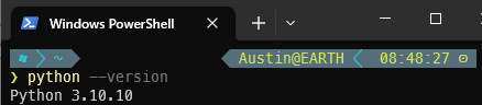
This is relatively straight-forward. To check your Python version, go to a command line and enter
python --version
If you already have Python 3.10.x installed (as seen in the screenshot below), you’re good to go (minor version doesn’t matter).
Python 3.10 installed for Stable Diffusion
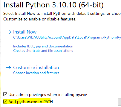
If not, go to the Python 3 download page and select the most recent 3.10 version. As of writing, the most recent is 3.10.10. Download the x64 installer and install. Ensure the “add python.exe to PATH” checkbox is checked. Adding python.exe to PATH means it can be called with only python at a command prompt instead of the full path, which is something like c:/users/whatever/somedirectory/moredirectories/3.10.10/python.exe.
Installing python and adding python.exe to PATH
2 – Installing Git (the source control system)
This is easier than Python – just install it – https://git-scm.com/downloads. Check for presence and version with git –version:
git installed and ready to go for Stable Diffusion
3 – Clone the Automatic1111 web UI (this is the front-end for using the various models)
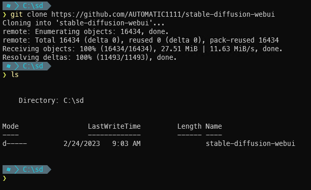
With Git, clone means to download a copy of the code repository. When you clone a repo, a new directory is created in whatever directory the command is run in. Meaning that if you navigate to your desktop, and run git clone xyz, you will have a new folder on your desktop named xyz with the contents of the repository. To keep things simple, I am going to create a folder for all my Stable Diffusion stuff in the C:/ root named sd and then clone into that folder.
After the git clone completes, there will be a new directory called ‘stable-diffusion-webui’:
stable-diffusion-webui cloned and ready to download models
4 – Download models
“Models” are what actually generate the content based on provided prompts. Generally, you will want to use pre-trained models. Luckily, there are many ready to use. Training your own model is far beyond the scope of this basic installation tutorial. Training your own models generally also requires huge amounts of time crunching numbers on very powerful GPUs.
As of writing, Stable Diffusion 1.5 (SD 1.5) is the recommended model. It can be downloaded (note: this is a 7.5GB file) from huggingface here.
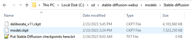
Take the downloaded file, and place it in the stable-diffusion-webui/models/Stable-diffusion directory and rename it to model.ckpt (it can be named anything you want but the web UI automatically attempts to load a model named ‘model.ckpt’ upon start). If you’re following along with the same directory structure as me, this file will end up at C:\sd\stable-diffusion-webui\models\Stable-diffusion\model.ckpt.
Another popular model is Deliberate. It can be downloaded (4.2GB) here. Put it in the same folder as the other model. No need to rename the 2nd (and other) models.
After downloading both models, the directory should look like this:
Stable Diffusion 1.5 (SD 1.5) and Deliberate_v11 models ready for use
5 – Adjust memory limits & enable listening outside of localhost (command line arguments)
Inside the main stable-diffusion-webui directory live a number of launcher files and helper files. Find webui-user.bat and edit it (.bat files can be right-clicked -> edit).
Add –medvram (two dashes) after the equals sign of COMMANDLINE_ARGS. If you also want the UI to listen on all IP addresses instead of just localhost (don’t do this unless you know what that means), also add –listen.
webui-user.bat after edits
@echo off

set PYTHON=
set GIT=
set VENV_DIR=
set COMMANDLINE_ARGS=--listen --medvram

call webui.bat
6 – First run
The UI tool (developed by automatic1111) will automatically download a variety of requirements upon first launch. It will take a few minutes to complete. Double-click the webui-user.bat file we just edited. It calls a few .bat files and eventually launches a Python file. The .bat files are essentially glue to stick a bunch of stuff together for the main file.
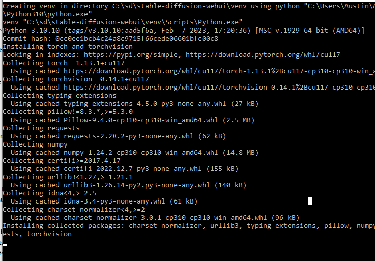
The very first thing it does is creates a Python venv (virtual environment) to keep the Stable Diffusion packages separate from your other Python packages. Then it pip installs a bunch of packages related to cuda/pytorch/numpy/etc so Python can interact with your GPU.
webui-user.bat using pip to install necessary python packages like cuda
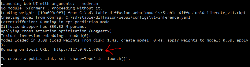
After everything is installed and ready to go, you will see a line that says: Running on local URL: http://127.0.0.1:7860. That means the Python web server UI is running on your own computer on port 7860 (if you added –listen to the launch args, it will show 0.0.0.0:7860, which means it is listening on all IP addresses and can be accessed by external machinse).
stable-diffusion-webui launched and ready to load
7 – Launching the web UI
With the web UI server running, it can be accessed via browser on the same computer running the Python at http://127.0.0.1:7860. That link should work for you if you click it.
Note that if the Python process closes for whatever reason (you close the command window, your computer reboots, etc), you need to double-click webui-user.bat to relaunch it and it needs to be running any time you want to access the web UI.
Automatic1111 stable diffusion web UI up and running
As seen in the screenshot, there are a ton of parameters/settings. I’ll highlight a few in the next section
8 – Generating Stable Diffusion images
This is the tricky part. The prompts make or break your generation. I am still learning. The prompt is where you enter what you want to see. Negative prompt is where you enter what you don’t want to see.
Let’s start simple, with cat in the prompt. Then click generate. A very reasonable-looking cat should soon appear (typically takes a couple seconds per image):
AI-generated cat with stable diffusion 1.5 with default settings
To highlight a few of the settings/sliders:
Stable diffusion checkpoint – model selector. Note that it’ll take a bit to load a new model (the multi-GB files need to be read in their entirety and ingested).
Prompt – what you want to see
Negative prompt – what you don’t want to see
Sampling method – various methods to sample new points
Sampling steps – how many iterations to use for image generation for a single image
Width – width of image to generate (in pixels). NOTE, you need a very powerful GPU with a ton of VRAM to go much higher than the default 512
Height – height of image to generate (in pixels). Same warning applies as width
Batch count – how many images to include in a batch generation
Batch size – haven’t used yet, presumably used to specify how many batches to generate
CFG Scale – this slider tells the models how specific they need to be for the prompt. Higher is more specific. Really high values (>12ish) start to get a bit abstract. Probably want to be in the range of 3-10 for this slider.
Seed – random number generator seed. -1 means use a new seed for every image.
Some thoughts on prompt/negative prompt
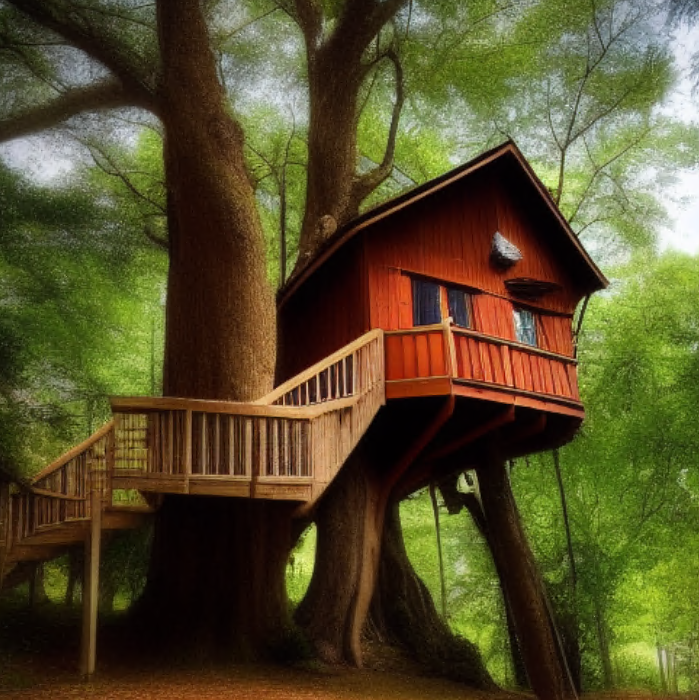
From my ~24 hours using this tool, it is very clear that prompt/negative prompts are what make or break your generation. I think that your ability as a pre-AI artist would come in handy here. I am no artist so I have a hard time putting what I want to see into words. Take example prompt: valley, fairytale treehouse village covered, matte painting, highly detailed, dynamic lighting, cinematic, realism, realistic, photo real, sunset, detailed, high contrast, denoised, centered. I would’ve said “fairytale treehouse” and stopped at that. Compare the two prompts below with the more detailed prompt directly below and the basic “fairytale treehouse” prompt after that:
AI-generated “fairytale treehouse” via stable diffusion. Prompt: valley, fairytale treehouse village covered, matte painting, highly detailed, dynamic lighting, cinematic, realism, realistic, photo real, sunset, detailed, high contrast, denoised, centeredAI-generated “fairytale treehouse” via stable diffusion. Prompt: fairytale treehouse
One of these looks perfectly in place for a fantasy story. The other you could very possibly see in person in a nearby forest.
Both positive and negative can get very long very quickly. Many of the AI-generated artifacts present over the last month or two can be eliminated with negative prompt entries.
I will not pretend to know what works well vs not. Google is your friend here. I believe that “prompt engineering” will be very important in AI’s future. Google is your friend here.
Conclusion
AI-generated content is here. It will not be going away. Even if it is outlawed, the code is out there. AI will be a huge part of our future, regardless of if you want it or not. As the saying goes – pandora’s box is now open.
I figured it was worth trying. The guide this is based off made it relatively easy for me (but I do have above-average computer skill), and I wanted to make it even easier. Hopefully you found this ‘how to set up stable diffusion’ guide easy to use as well. Please let me know in the comments section if you have any questions/comments/feedback – I check at least daily!
Resources
Huge shout out to whoever wrote the guide (“all anons”) at https://rentry.org/voldy. That is essentially where this entire guide came from.