Tag: ADS-B

I’ve been building SkySpottr, an AR app overlaying aircraft information on your phone’s screen, using your device’s location, orientation, and incoming aircraft data (ADS-B) to predict where planes should appear on screen, then uses a YOLO model to lock onto the actual aircraft and refine the overlay. YOLOv8 worked great for this… until I actually read the license.

Welcome to Austin’s Nerdy Things, where we train from scratch entire neural networks to avoid talking to lawyers.

The Problem with Ultralytics

YOLOvWhatver is excellent. Fast, accurate, easy to use, great documentation. But Ultralytics licenses it under AGPL-3.0, which means if you use it in a product, you either need to open-source your entire application or pay for a commercial license. For a side project AR app that I might eventually monetize? That’s a hard pass.

Enter YOLOX from Megvii (recommended by either ChatGPT or Claude, can’t remember which, as an alternative). MIT licensed. Do whatever you want with it. The catch? You have to train your own models from scratch instead of using Ultralytics’ pretrained weights and easy fine-tuning pipeline. I have since learned there are some pretrained models. I didn’t use them.

So training from scratch is what I did. Over a few late nights in December 2025, I went from zero YOLOX experience to running custom-trained aircraft detection models in my iOS app. Here’s how it went.

The Setup

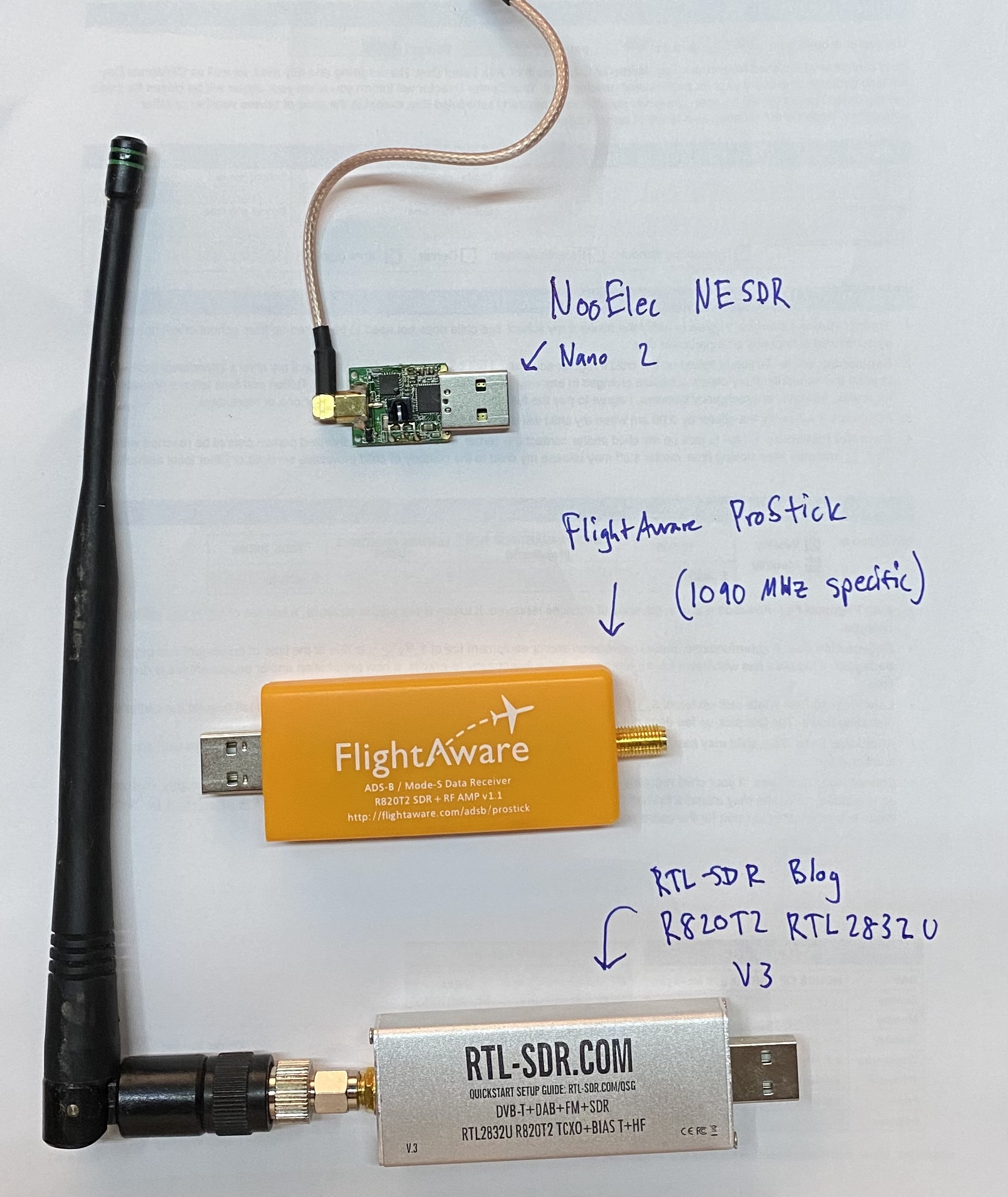
Hardware: RTX 3090 on my Windows machine, COCO2017 dataset on network storage (which turned out to be totally fine for training speed), and way too many terminal windows open.

I started with the official YOLOX repo and the aircraft class from COCO2017. The dataset has about 3,000 training images with airplanes, which is modest but enough to get started.

git clone https://github.com/Megvii-BaseDetection/YOLOX
pip install -v -e .

The first training run failed immediately because I forgot to install YOLOX as a package. Classic. Then it failed again because I was importing a class that didn’t exist in the version I had. Claude (who was helping me through this, and hallucinated said class) apologized and fixed the import. We got there eventually.

Training Configs: Nano, Tiny, Small, and “Nanoish”

YOLOX has a nice inheritance-based config system. You create a Python file, inherit from a base experiment class, and override what you want. I ended up with four different configs:

• yolox_nano_aircraft.py – The smallest. 0.9M params, 1.6 GFLOPs. Runs on anything.
• yolox_tiny_aircraft.py – Slightly bigger with larger input size for small object detection.
• yolox_small_aircraft.py – 5M params, 26 GFLOPs. The “serious” model.
• yolox_nanoish_aircraft.py – My attempt at something between nano and tiny.

The “nanoish” config was my own creation where I tried to find a sweet spot. I bumped the width multiplier from 0.25 to 0.33 and… immediately got a channel mismatch error because 0.33 doesn’t divide evenly into the architecture. Turns out you can’t just pick arbitrary numbers. I am a noob at these things. Lesson learned.

After some back-and-forth, I settled on a config with 0.3125 width (which is 0.25 \* 1.25, mathematically clean) and 512×512 input. This gave me roughly 1.2M params – bigger than nano, smaller than tiny, and it actually worked.

Here’s the small model config – the one that ended up in production. The key decisions are width = 0.50 (2x wider than nano for better feature extraction), 640×640 input for small object detection, and full mosaic + mixup augmentation:

class Exp(MyExp):
    def __init__(self):
        super(Exp, self).__init__()

        # Model config - YOLOX-Small architecture
        self.num_classes = 1  # Single class: airplane
        self.depth = 0.33
        self.width = 0.50  # 2x wider than nano for better feature extraction

        # Input/output config - larger input helps small object detection
        self.input_size = (640, 640)
        self.test_size = (640, 640)
        self.multiscale_range = 5  # Training will vary from 480-800

        # Data augmentation
        self.mosaic_prob = 1.0
        self.mosaic_scale = (0.1, 2.0)
        self.enable_mixup = True
        self.mixup_prob = 1.0
        self.flip_prob = 0.5
        self.hsv_prob = 1.0

        # Training config
        self.warmup_epochs = 5
        self.max_epoch = 400
        self.no_aug_epochs = 100
        self.basic_lr_per_img = 0.01 / 64.0
        self.scheduler = "yoloxwarmcos"

    def get_model(self):
        from yolox.models import YOLOX, YOLOPAFPN, YOLOXHead

        in_channels = [256, 512, 1024]
        # Small uses standard convolutions (no depthwise)
        backbone = YOLOPAFPN(self.depth, self.width, in_channels=in_channels, act=self.act)
        head = YOLOXHead(self.num_classes, self.width, in_channels=in_channels, act=self.act)
        self.model = YOLOX(backbone, head)
        return self.model

And the nanoish config for comparison – note the depthwise=True and the width of 0.3125 (5/16) that I landed on after the channel mismatch debacle:

class Exp(MyExp):
    def __init__(self):
        super(Exp, self).__init__()

        self.num_classes = 1
        self.depth = 0.33
        self.width = 0.3125  # 5/16 - halfway between nano (0.25) and tiny (0.375)

        self.input_size = (512, 512)
        self.test_size = (512, 512)

        # Lighter augmentation than small - this model is meant to be fast
        self.mosaic_prob = 0.5
        self.mosaic_scale = (0.5, 1.5)
        self.enable_mixup = False

    def get_model(self):
        from yolox.models import YOLOX, YOLOPAFPN, YOLOXHead

        in_channels = [256, 512, 1024]
        backbone = YOLOPAFPN(self.depth, self.width, in_channels=in_channels,
                             act=self.act, depthwise=True)  # Depthwise = lighter
        head = YOLOXHead(self.num_classes, self.width, in_channels=in_channels,
                         act=self.act, depthwise=True)
        self.model = YOLOX(backbone, head)
        return self.model

Training is then just:

python tools/train.py -f yolox_small_aircraft.py -d 1 -b 16 --fp16 -c yolox_s.pth

The -c yolox_s.pth loads YOLOX’s pretrained COCO weights as a starting point (transfer learning). The -d 1 is one GPU, -b 16 is batch size 16 (about 8GB VRAM on the 3090 with fp16), and --fp16 enables mixed precision training.

The Small Object Problem

Here’s the thing about aircraft detection for an AR app: planes at cruise altitude look tiny. A 747-8 at 37,000 feet is maybe 20-30 pixels on your phone screen if you’re lucky, even with the 4x optical zoom of the newest iPhones (8x for the 12MP weird zoom mode). Standard YOLO models are tuned for reasonable-sized objects, not specks in the sky. The COCO dataset has aircraft that are reasonably sized, like when you’re sitting at your gate at an airport and take a picture of the aircraft 100 ft in front of you.

My first results were underwhelming. The nano model was detecting larger aircraft okay but completely missing anything at altitude. The evaluation metrics looked like this:

AP for airplane = 0.234
AR for small objects = 0.089

Not great. The model was basically only catching aircraft on approach or takeoff.

For the small config, I made some changes to help with tiny objects:

• Increased input resolution to 640×640 (more pixels = more detail for small objects)
• Enabled full mosaic and mixup augmentation (helps the model see varied object scales)
• Switched from depthwise to regular convolutions (more capacity)
• (I’ll be honest, I was leaning heavily on Claude for the ML-specific tuning decisions here)

This pushed the model to 26 GFLOPs though, which had me worried about phone performance.

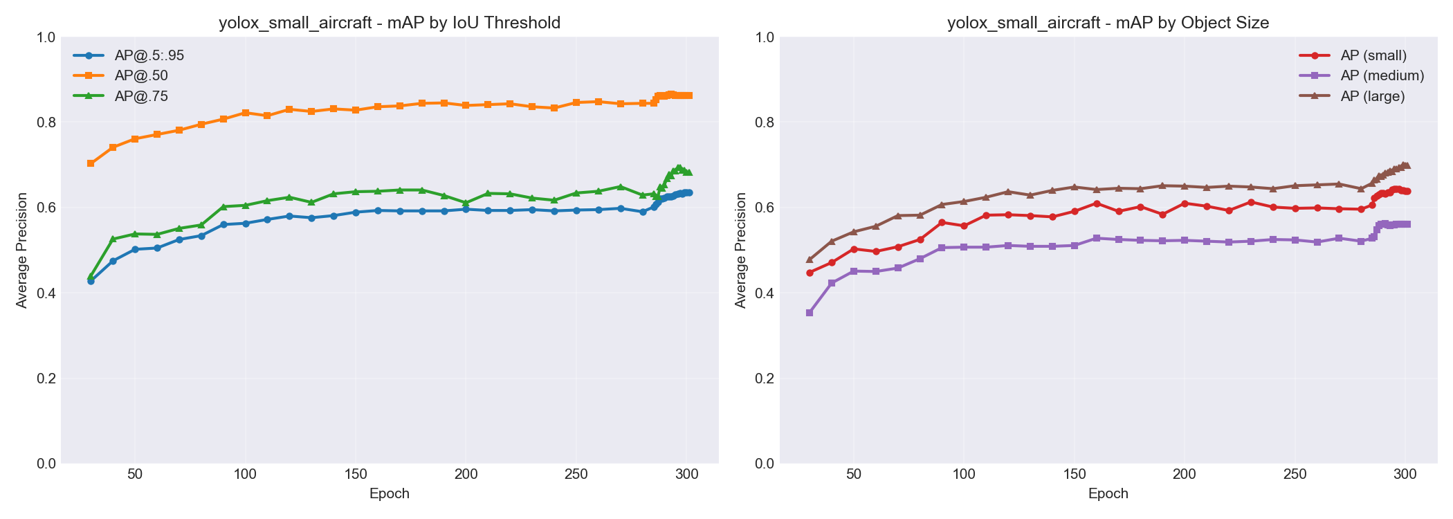
Here’s what the small model’s accuracy looked like broken down by object size. You can see AP for small objects climbing from ~0.45 to ~0.65 over training, while large objects hit ~0.70. Progress, but small objects remain the hardest category – which tracks with the whole “specks in the sky” problem.

Will This Actually Run on a Phone?

The whole point of this exercise was to run inference on an iPhone. So here is some napkin math:

Model	GFLOPs	Estimated Phone Inference
Nano	1.6	~15ms, smooth 30fps easy
Nanoish	3.2	~25ms, still good
Small	26	~80ms, might be sluggish
YOLOv8n (for reference)	8.7	~27ms

My app was already running YOLOv8n at 15fps with plenty of headroom. So theoretically even the small model should work, but nano/nanoish would leave more room for everything else the app needs to do.

The plan: train everything, compare accuracy, quantize for deployment, and see what actually works in practice.

Training Results (And a Rookie Mistake)

After letting things run overnight (300 epochs takes a while even on a 3090), here’s what I got:

The nanoish model at epoch 100 was already showing 94% detection rate on test images, beating the fully-trained nano model. And it wasn’t even done training yet.

Quick benchmark on 50 COCO test images with aircraft (RTX 3090 GPU inference – not identical to phone, but close enough for the smaller models to be representative):

Model	Detection Rate	Avg Detections/Image	Avg Inference (ms)	FPS
YOLOv8n	58.6%	0.82	33.6	29.7
YOLOX nano	74.3%	1.04	14.0	71.4
YOLOX nanoish	81.4%	1.14	15.0	66.9
YOLOX tiny	91.4%	1.28	16.5	60.7
YOLOX small	92.9%	1.30	17.4	57.4
Ground Truth	–	1.40	–	–

YOLOv8n getting beaten by every single YOLOX variant while also being slower was… not what I expected. Here’s the mAP comparison across all the models over training – you can see the hierarchy pretty clearly:

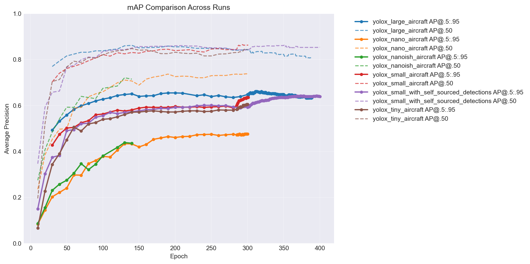
The big takeaway: more capacity = better accuracy, but with diminishing returns. The jump from nano to nanoish is huge, nanoish to small is solid, and tiny lands somewhere in between depending on the epoch. (You’ll notice two extra lines in the chart – a large model and a self-sourced variant. I kept training after this post’s story ends. More on the self-sourced pipeline later. You can also see the large model is clearly overfitting past epoch ~315 – loss keeps decreasing but mAP starts dropping. My first time overfitting a model.)

The nanoish model hit a nice sweet spot. Faster than YOLOv8n, better small object detection than pure nano, and still lightweight enough for mobile.

And here is the output from my plot_training.py script:

============================================================
SUMMARY
============================================================
Run                         Epochs   Final Loss    Best AP  Best AP50
------------------------------------------------------------
yolox_large_aircraft           391       0.6000     0.6620     0.8620
yolox_nano_aircraft            300       3.3000     0.4770     0.7390
yolox_nanoish_aircraft         142       4.3000     0.4390     0.7210
yolox_small_aircraft           302       2.2000     0.6360     0.8650
yolox_small_with_self_sou      400       1.4000     0.6420     0.8620
yolox_tiny_aircraft            300       2.5000     0.6060     0.8480
============================================================

====================================================================================================
mAP VALUES AT SPECIFIC EPOCHS
====================================================================================================
Run                           AP@280     AP50@280    APsmall@280     AP@290     AP50@290    APsmall@290     AP@299     AP50@299    APsmall@299
----------------------------------------------------------------------------------------------------
yolox_large_aircraft          0.6350       0.8410         0.6690     0.6390       0.8410         0.6750 0.6480(300)       0.8440         0.6780
yolox_nano_aircraft           0.4750       0.7360         0.4000     0.4740       0.7360         0.3970     0.4770       0.7380         0.4030
yolox_nanoish_aircraft           N/A          N/A            N/A        N/A          N/A            N/A        N/A          N/A            N/A
yolox_small_aircraft          0.5900       0.8440         0.5960     0.6230       0.8610         0.6340     0.6360       0.8630         0.6410
yolox_small_with_self_sou     0.5940       0.8430         0.5690     0.5900       0.8420         0.5660 0.5930(300)       0.8420         0.5630
yolox_tiny_aircraft           0.5800       0.8300         0.5650     0.5950       0.8340         0.5830     0.6060       0.8440         0.5780
====================================================================================================

But there was a problem I didn’t notice until later: my training dataset had zero images without aircraft in them. Every single training image contained at least one airplane. This is… not ideal if you want your model to learn what an airplane isn’t. More on that shortly.

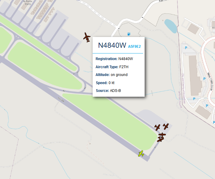
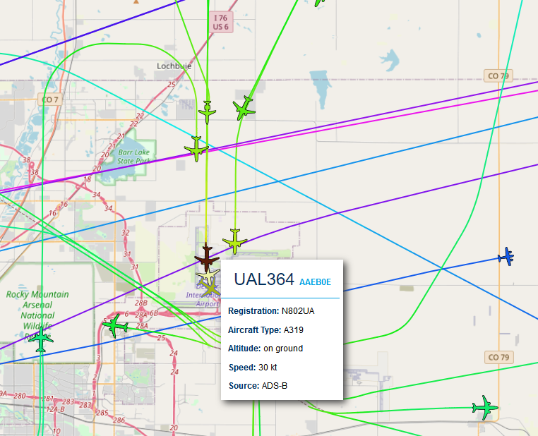
How It Actually Works in the App

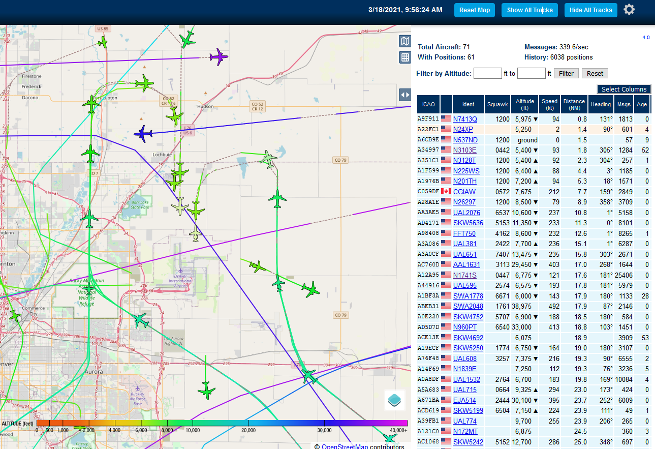
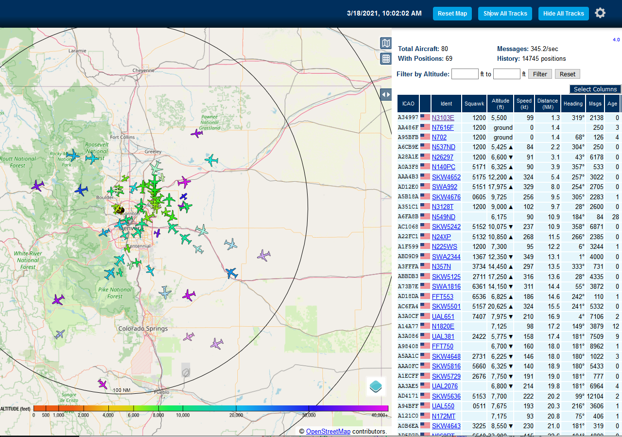
Before I get to results, here’s what the ML is actually doing in SkySpottr. The app combines multiple data sources to track aircraft:

1. ADS-B data tells us where aircraft are in 3D space (lat, lon, altitude)
2. Device GPS and orientation tell us where the phone is and which way it’s pointing
3. Physics-based prediction places aircraft overlays on screen based on all the above

That prediction is usually pretty good, but phone sensors drift and aircraft positions are slightly delayed. So the overlays can be off by a couple degrees. This is where YOLO comes in.

The app runs the model on each camera frame looking for aircraft. When it finds one within a threshold distance of where the physics engine predicted an aircraft should be, it “snaps” the overlay to the actual detected position. The UI shows an orange circle around the aircraft and marks it as “SkySpottd” – confirmed via machine learning.

I call this “ML snap” mode. It’s the difference between “there’s probably a plane somewhere around here” and “that specific bright dot is definitely the aircraft.”

The model runs continuously on device, which is why inference time matters so much. Even at 15fps cap, that’s still 15 inference cycles per second competing with everything else the app needs to do (sensor fusion, WebSocket data, AR rendering, etc.). Early on I was seeing 130%+ CPU usage on my iPhone, which is not great for battery life. Every millisecond saved on inference is a win.

Getting YOLOX into CoreML

One thing the internet doesn’t tell you: YOLOX and Apple’s Vision framework don’t play nice together.

YOLOv8 exports to CoreML with a nice Vision-compatible interface. You hand it an image, it gives you detections. Easy. YOLOX expects different preprocessing – it wants pixel values in the 0-255 range (not normalized 0-1), and the output tensor layout is different.

The conversion pipeline goes PyTorch → TorchScript → CoreML. Here’s the core of it:

import torch
import coremltools as ct
from yolox.models import YOLOX, YOLOPAFPN, YOLOXHead

# Build model (same architecture as training config)
backbone = YOLOPAFPN(depth=0.33, width=0.50, in_channels=[256, 512, 1024], act="silu")
head = YOLOXHead(num_classes=1, width=0.50, in_channels=[256, 512, 1024], act="silu")
model = YOLOX(backbone, head)

# Load trained weights
ckpt = torch.load("yolox_small_best.pth", map_location="cpu", weights_only=False)
model.load_state_dict(ckpt["model"])
model.eval()
model.head.decode_in_inference = True  # Output pixel coords, not raw logits

# Trace and convert
dummy = torch.randn(1, 3, 640, 640)
traced = torch.jit.trace(model, dummy)
mlmodel = ct.convert(
    traced,
    inputs=[ct.TensorType(name="images", shape=(1, 3, 640, 640))],
    outputs=[ct.TensorType(name="output")],
    minimum_deployment_target=ct.target.iOS15,
    convert_to="mlprogram",
)
mlmodel.save("yolox_small_aircraft.mlpackage")

The decode_in_inference = True is crucial — without it, the model outputs raw logits and you’d need to implement the decode head in Swift. With it, the output is [1, N, 6] where 6 is [x_center, y_center, width, height, obj_conf, class_score] in pixel coordinates.

On the Swift side, Claude ended up writing a custom detector that bypasses the Vision framework entirely. Here’s the preprocessing — the part that was hardest to get right:

/// Convert pixel buffer to MLMultiArray [1, 3, H, W] with 0-255 range
private func preprocess(pixelBuffer: CVPixelBuffer) -> MLMultiArray? {
    // GPU-accelerated resize via Core Image
    let ciImage = CIImage(cvPixelBuffer: pixelBuffer)
    let scaleX = CGFloat(inputSize) / ciImage.extent.width
    let scaleY = CGFloat(inputSize) / ciImage.extent.height
    let scaledImage = ciImage.transformed(by: CGAffineTransform(scaleX: scaleX, y: scaleY))

    // Reuse pixel buffer from pool (memory leak fix #1)
    var resizedBuffer: CVPixelBuffer?
    CVPixelBufferPoolCreatePixelBuffer(kCFAllocatorDefault, pool, &resizedBuffer)
    guard let buffer = resizedBuffer else { return nil }
    ciContext.render(scaledImage, to: buffer)

    // Reuse pre-allocated MLMultiArray (memory leak fix #2)
    guard let array = inputArray else { return nil }

    CVPixelBufferLockBaseAddress(buffer, .readOnly)
    defer { CVPixelBufferUnlockBaseAddress(buffer, .readOnly) }

    let bytesPerRow = CVPixelBufferGetBytesPerRow(buffer)
    let pixels = CVPixelBufferGetBaseAddress(buffer)!.assumingMemoryBound(to: UInt8.self)
    let arrayPtr = array.dataPointer.assumingMemoryBound(to: Float.self)
    let channelStride = inputSize * inputSize

    // BGRA → RGB, keep 0-255 range (YOLOX expects unnormalized pixels)
    // Direct pointer access is ~100x faster than MLMultiArray subscript
    for y in 0..<inputSize {
        let rowOffset = y * bytesPerRow
        let yOffset = y * inputSize
        for x in 0..<inputSize {
            let px = rowOffset + x * 4
            let idx = yOffset + x
            arrayPtr[idx] = Float(pixels[px + 2])                      // R
            arrayPtr[channelStride + idx] = Float(pixels[px + 1])      // G
            arrayPtr[2 * channelStride + idx] = Float(pixels[px])      // B
        }
    }
    return array
}

The two key gotchas: (1) BGRA byte order from the camera vs RGB that the model expects, and (2) YOLOX wants raw 0-255 pixel values, not the 0-1 normalized range that most CoreML models expect. If you normalize, everything silently breaks — the model runs, returns garbage, and you spend an evening wondering why.

For deployment, I used CoreML’s INT8 quantization (coremltools.optimize.coreml.linear_quantize_weights). This shrinks the model by about 50% with minimal accuracy loss. The small model went from ~17MB to 8.7MB, and inference time improved slightly.

Real World Results (Round 1)

I exported the nanoish model and got it running in SkySpottr. The good news: it works. The ML snap feature locks onto aircraft, the orange verification circles appear, and inference is fast enough that I don’t notice any lag.

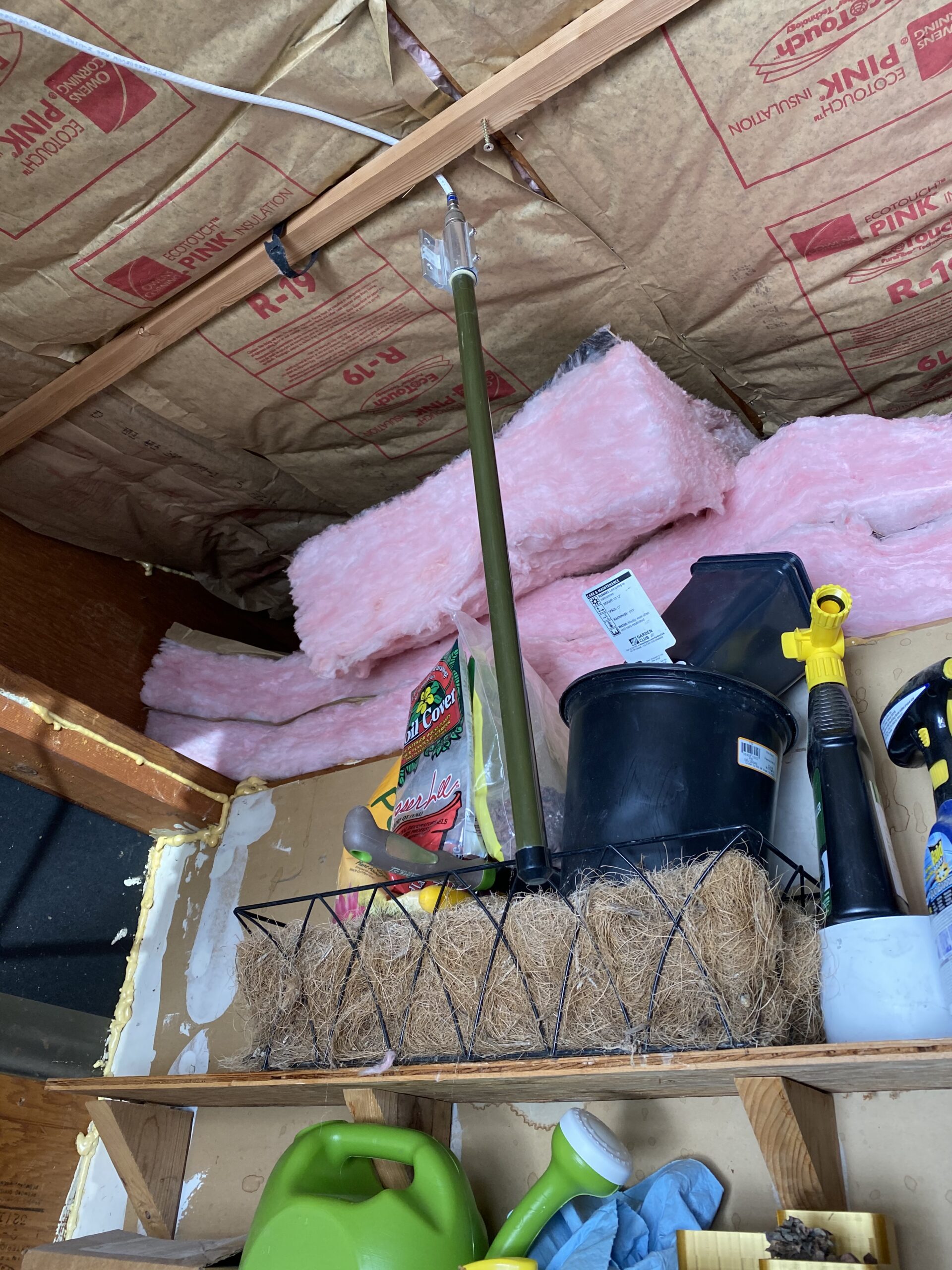
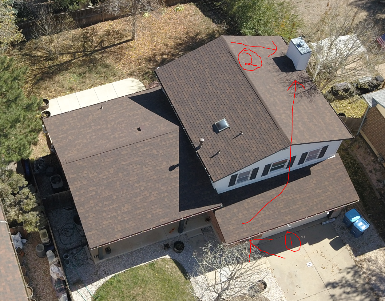
The less good news: false positives. Trees, parts of houses, certain cloud formations – the model occasionally thinks these are aircraft. Remember that rookie mistake about no negative samples? Yeah.

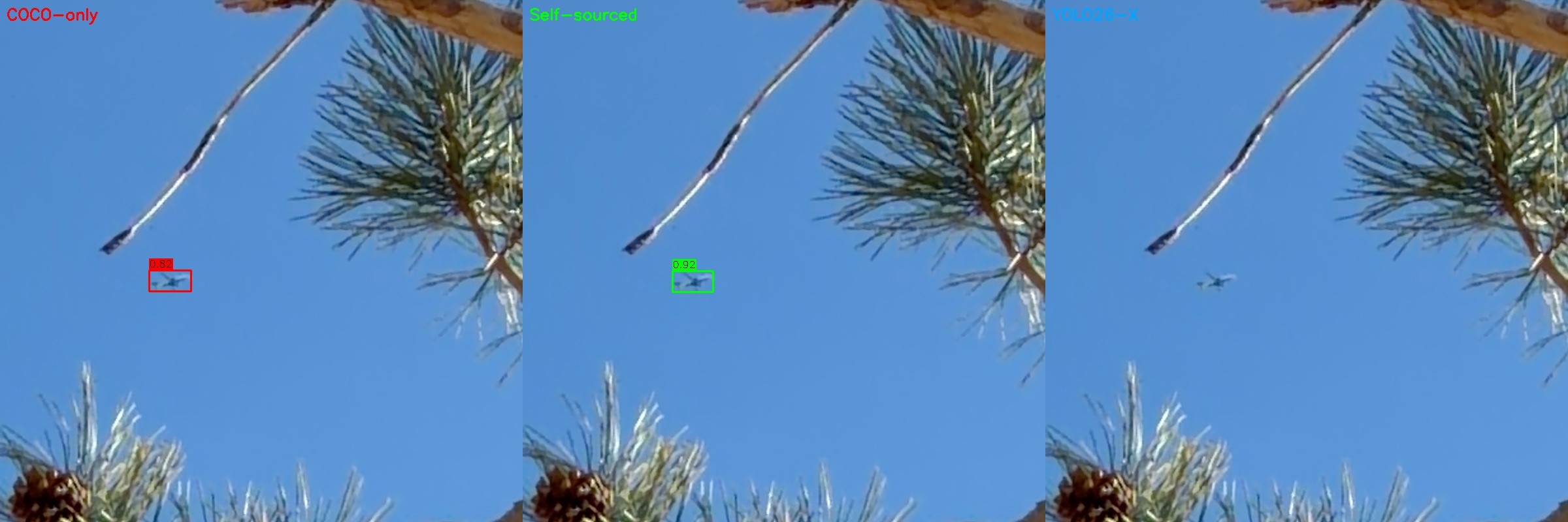
I later set up a 3-way comparison to visualize exactly this kind of failure. The three panels show my COCO-only trained model (red boxes), a later model trained on self-sourced images (green boxes – I’ll explain this pipeline shortly), and YOLO26-X as a ground truth oracle (right panel, no boxes means no detection). The COCO-only model confidently detects an “aircraft” that is… a building. The other two correctly ignore it.

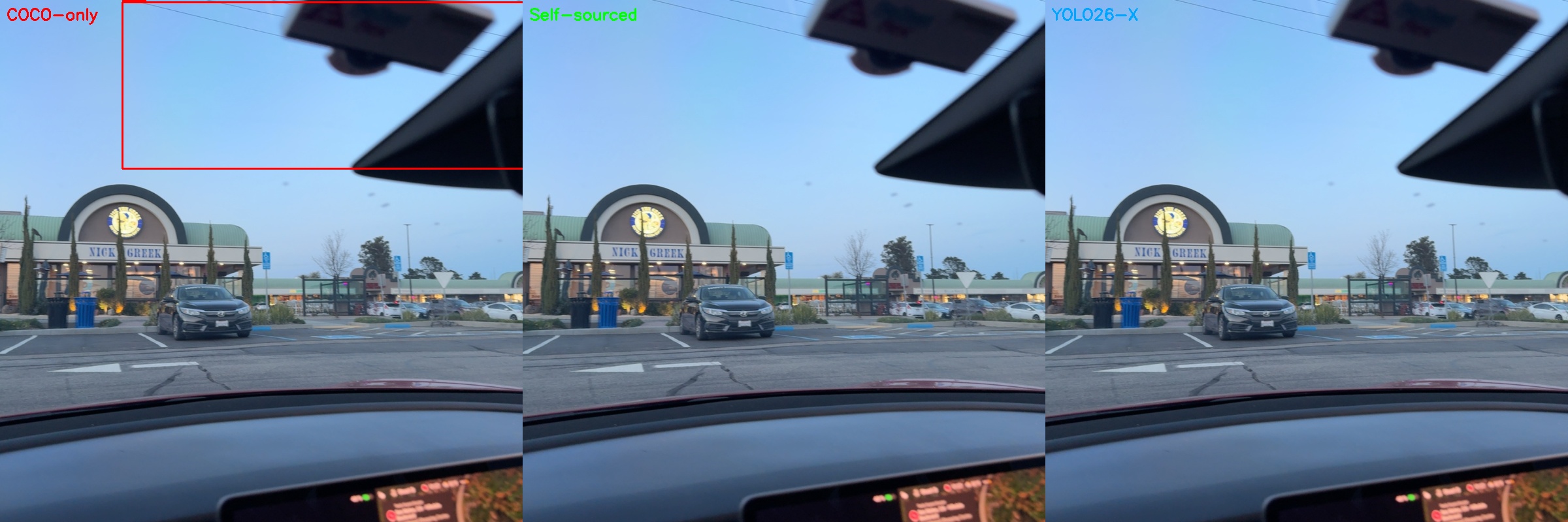
The app handles this gracefully because of the matching threshold. Random false positives in empty sky don’t trigger the snap because there’s no predicted aircraft nearby to match against. But when there’s a tree branch right next to where a plane should be, the model sometimes locks onto the wrong thing.

The even less good news: it still struggles with truly distant aircraft. A plane at 35,000 feet that’s 50+ miles away is basically a single bright pixel. No amount of ML is going to reliably detect that. For those, the app falls back on pure ADS-B prediction, which is usually good enough to get the overlay in the right general area.

But when it works, it works. I’ll show some examples of successful detections in the self-sourced section below.

The Memory Leak Discovery (Fun Debugging Tangent)

While testing the YOLOX integration, I was also trying to get RevenueCat working for subscriptions. Had the app running for about 20 minutes while I debugged the in-app purchase flow. Noticed it was getting sluggish, opened Instruments, and… yikes.

Base memory for the app is around 200MB. After 20 minutes of continuous use, it had climbed to 450MB. Classic memory leak pattern.

The culprit was AI induced, and AI resolved: it was creating a new CVPixelBuffer and MLMultiArray for every single frame. At 15fps, that’s 900 allocations per minute that weren’t getting cleaned up fast enough.

The fix was straightforward – use a CVPixelBufferPool for the resize buffers and pre-allocate a single MLMultiArray that gets reused. Memory now stays flat even after hours of use.

(The RevenueCat thing? I ended up ditching it entirely and going with native StoreKit2. RevenueCat is great, but keeping debug and release builds separate was more hassle than it was worth for a side project. StoreKit2 is actually pretty nice these days if you don’t need the analytics. I’m at ~80 downloads, and not a single purchase. First paid app still needs some fine tuning, clearly, on the whole freemium thing.)

Round 2: Retraining with Negative Samples

After discovering the false positive issue, I went back and retrained. This time I made sure to include images without aircraft – random sky photos, clouds, trees, buildings, just random COCO2017 stuff. The model needs to learn what’s NOT an airplane just as much as what IS one.

Here’s the extraction script that handles the negative sampling. The key insight: you need to explicitly tell the model what empty sky looks like:

def extract_airplane_dataset(split="train", negative_ratio=0.2, seed=42):
    """Extract airplane images from COCO, with negative samples."""
    with open(f"instances_{split}2017.json") as f:
        coco_data = json.load(f)

    # Find all images WITH airplanes
    airplane_image_ids = set()
    for ann in coco_data['annotations']:
        if ann['category_id'] == AIRPLANE_CATEGORY_ID:  # 5 in COCO
            airplane_image_ids.add(ann['image_id'])

    # Find images WITHOUT airplanes for negative sampling
    all_ids = {img['id'] for img in coco_data['images']}
    negative_ids = all_ids - airplane_image_ids

    # Add 20% negative images (no airplanes = teach model what ISN'T a plane)
    num_negatives = int(len(airplane_image_ids) * negative_ratio)
    sampled_negatives = random.sample(list(negative_ids), num_negatives)
    # ... copy images and annotations to output directory

I also switched from nanoish to the small model. The accuracy improvement on distant aircraft was worth the extra compute, and with INT8 quantization the inference time came in at around 5.6ms on an iPhone – way better than my napkin math predicted. Apple’s Neural Engine is impressive.

The final production model: YOLOX-Small, 640×640 input, INT8 quantized, ~8.7MB on disk. It runs at 15fps with plenty of headroom for the rest of the app on my iPhone 17 Pro.

Round 3: Self-Sourced Images and Closing the Loop

So the model works, but it was trained entirely on COCO2017 – airport tarmac photos, stock images, that kind of thing. My app is pointing at the sky from the ground. Those are very different domains.

I added a debug flag to SkySpottr for my phone that saves every camera frame where the model fires a detection. Just flip it on, walk around outside for a while, and the app quietly collects real-world training data. Over a few weeks of casual use, I accumulated about 2,000 images from my phone.

The problem: these images don’t have ground truth labels. I’m not going to sit there and manually draw bounding boxes on 2,000 sky photos. So I used YOLO26-X (Ultralytics’ latest and greatest, which I’m fine using as an offline tool since it never ships in the app) as a teacher model. Run it on all the collected images, take its high-confidence detections as pseudo-labels, convert to COCO annotation format, and now I have a self-sourced dataset to mix in with the original COCO training data.

Here’s the pseudo-labeling pipeline. First, run the teacher model on all collected images:

from ultralytics import YOLO

model = YOLO("yolo26x.pt")  # Big model, accuracy over speed

for img_path in tqdm(image_paths, desc="Processing images"):
    results = model(str(img_path), conf=0.5, verbose=False)
    boxes = results[0].boxes
    airplane_boxes = boxes[boxes.cls == AIRPLANE_CLASS_ID]

    for box in airplane_boxes:
        xyxy = box.xyxy[0].cpu().numpy().tolist()
        x1, y1, x2, y2 = xyxy
        detections.append({
            "bbox_xywh": [x1, y1, x2 - x1, y2 - y1],  # COCO format
            "confidence": float(box.conf[0]),
        })

Then convert those detections to COCO annotation format so YOLOX can train on them:

def convert_to_coco(detections):
    """Convert YOLO26 detections to COCO training format."""
    coco_data = {
        "images": [], "annotations": [],
        "categories": [{"id": 1, "name": "airplane", "supercategory": "vehicle"}],
    }

    for uuid, data in detections.items():
        img_path = Path(data["image_path"])
        width, height = Image.open(img_path).size

        if width > 1024 or height > 1024:  # Skip oversized images
            continue

        coco_data["images"].append({"id": image_id, "file_name": f"{uuid}.jpg",
                                     "width": width, "height": height})

        for det in data["detections"]:
            coco_data["annotations"].append({
                "id": ann_id, "image_id": image_id, "category_id": 1,
                "bbox": det["bbox_xywh"], "area": det["bbox_xywh"][2] * det["bbox_xywh"][3],
                "iscrowd": 0,
            })

    with open("instances_train.json", "w") as f:
        json.dump(coco_data, f)

Finally, combine both datasets in the training config using YOLOX’s ConcatDataset:

def get_dataset(self, cache=False, cache_type="ram"):
    from yolox.data import COCODataset, TrainTransform
    from yolox.data.datasets import ConcatDataset

    preproc = TrainTransform(max_labels=50, flip_prob=0.5, hsv_prob=1.0)

    # Original COCO aircraft dataset
    coco_dataset = COCODataset(data_dir=self.data_dir, json_file=self.train_ann,
                                img_size=self.input_size, preproc=preproc, cache=cache)

    # Self-sourced dataset (YOLO26-X validated)
    self_sourced = COCODataset(data_dir=self.self_sourced_dir, json_file=self.self_sourced_ann,
                                name="train", img_size=self.input_size, preproc=preproc, cache=cache)

    print(f"COCO aircraft images: {len(coco_dataset)}")
    print(f"Self-sourced images: {len(self_sourced)}")
    return ConcatDataset([coco_dataset, self_sourced])

Out of 2,000 images, YOLO26-X found aircraft in about 108 of them at a 0.5 confidence threshold – a 1.8% hit rate, which makes sense since most frames are just empty sky between detections. I filtered out anything over 1024px and ended up with a nice supplementary dataset of aircraft-from-the-ground images.

The 3-way comparison images I showed earlier came from this pipeline. Here’s what successful detections look like – the COCO-only model (red), self-sourced model (green), and YOLO26-X (right panel, shown at full resolution so you can see what we’re actually detecting):

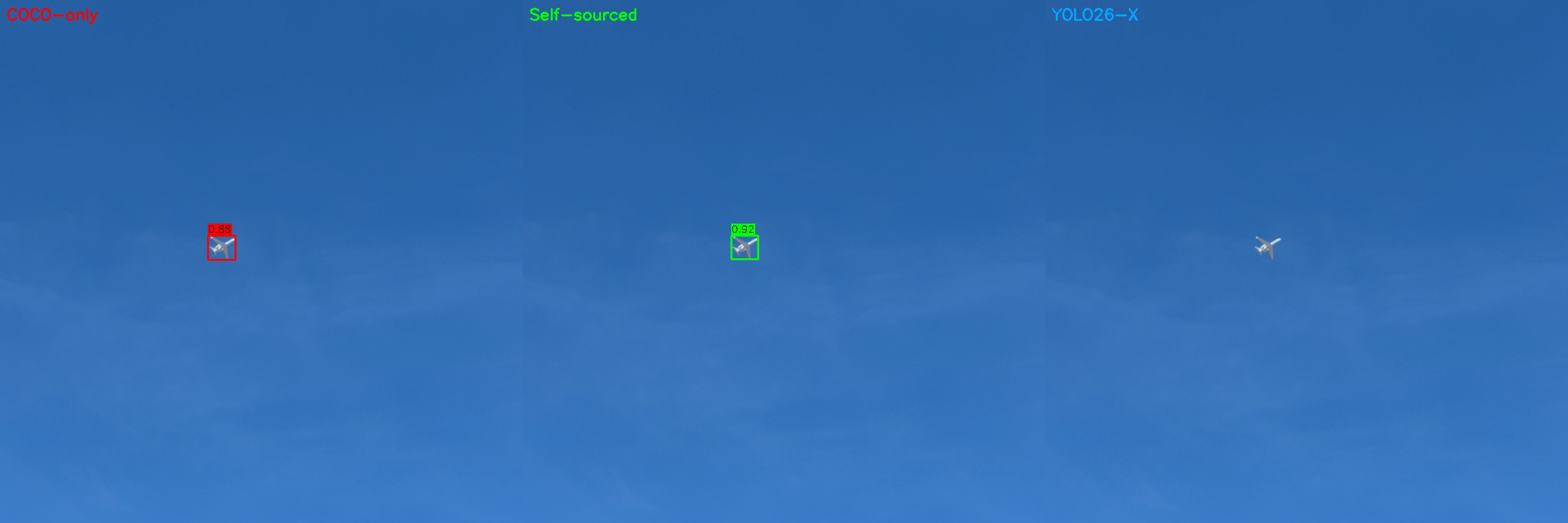
That’s maybe 30 pixels of airplane against blue sky, detected with 0.88 and 0.92 confidence by the two YOLOX variants.

And here’s one I particularly like – aircraft spotted through pine tree branches. Real-world conditions, not a clean test image. Both YOLOX models nail it, YOLO26-X misses at this confidence threshold:

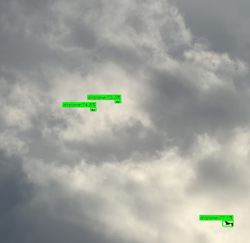
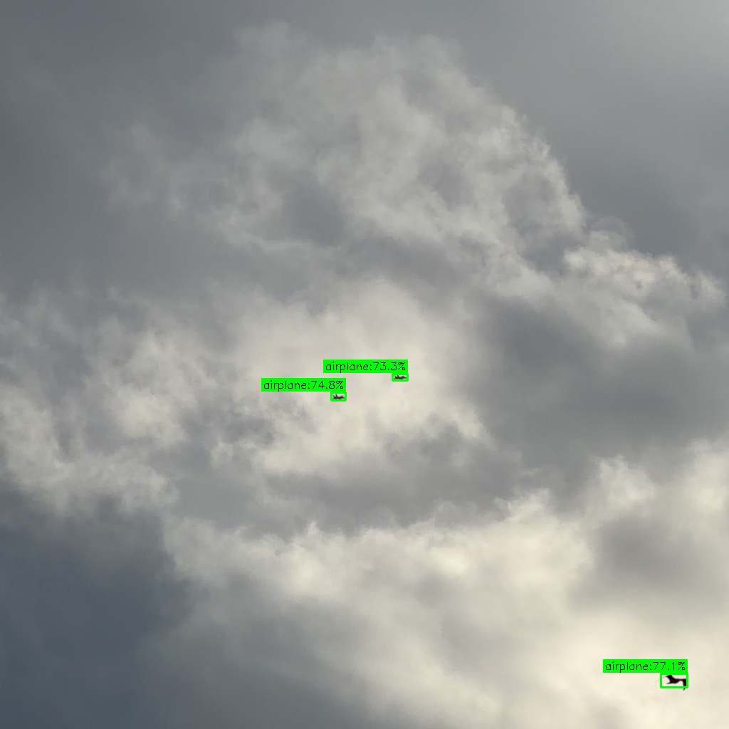
And a recent one from February 12, 2026 – a pair of what appear to be F/A-18s over Denver at 4:22 PM MST, captured at 12x zoom. The model picks up both jets at 73-75% confidence, plus the bird in the bottom-right at 77% (a false positive the app filters out via ADS-B matching). Not bad for specks against an overcast sky.

I also trained a full YOLOX-Large model (depth 1.0, width 1.0, 1024×1024 input) on the combined dataset, just to see how far I could push it. Too heavy for phone deployment, but useful for understanding the accuracy ceiling.

Conclusion

Was this worth it to avoid Ultralytics’ licensing? Since it took an afternoon and a couple evenings of vibe-coding, yes, it was not hard to switch. Not just because MIT is cleaner than AGPL, but because I learned a ton about how these models actually work. The Ultralytics ecosystem is so polished that it’s easy to treat it as a black box. Building from YOLOX forced me to understand some of the nuances, the training configs, and the tradeoffs between model size and accuracy.

Plus, I can now say I trained my own object detection model from scratch. That’s worth something at parties. Nerdy parties, anyway.

SkySpottr is live on the App Store if you want to see the model in action – point your phone at the sky and watch it lock onto aircraft in real-time.

The self-sourced pipeline is still running. Every time I use the app with the debug flag on, it collects more training data. The plan is to periodically retrain as the dataset grows – especially now that I’m getting images from different weather conditions, times of day, and altitudes. The COCO-only model was a solid start, but a model trained on actual ground-looking-up images of aircraft at altitude? That’s the endgame.