I revisited my Python X-Plane autopilot a few weeks ago because it was pretty clunky for how to adjust setpoints and such. The job I started 1.5 years ago is exclusively Python, so I wanted to redo a bit.
Quick aside: For the new PC I just built – Ryzen 9 7900x, 2x32GB 6000 MHz, etc, X-Plane 10 was the 2nd “game” I installed on it. The first was Factorio (I followed Nilaus’ megabase in a book and have got to 5k SPM). Haven’t tried the newer sims yet, but I think they’ll still be somewhat limited by my RTX 2080 Super.
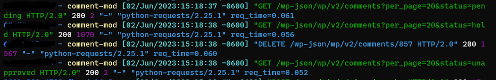
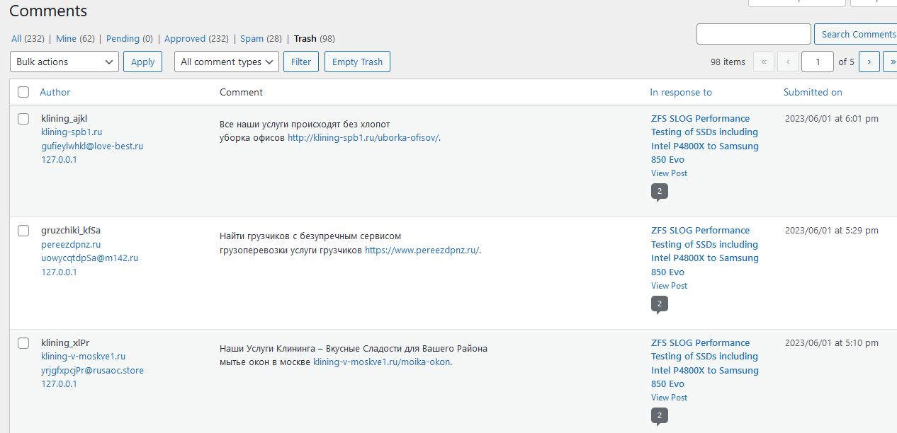
Well imagine my surprise when I woke up to 6x the normal daily hits by 7am. I checked the weblogs and found that my post was trending on ycombinator.com (Hacker News). So I am going to skip pretty much all background and just post the updated code for now, and will go back and clean up this post at some point.
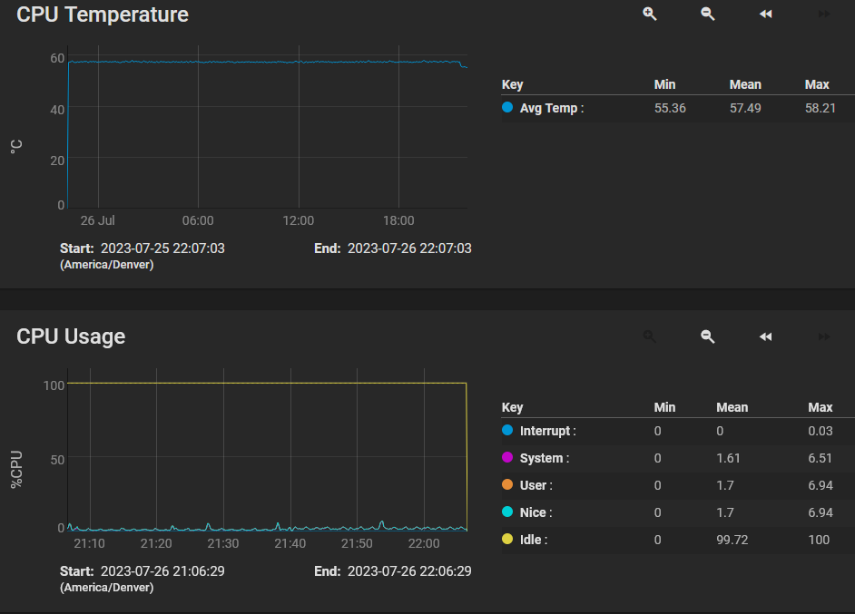
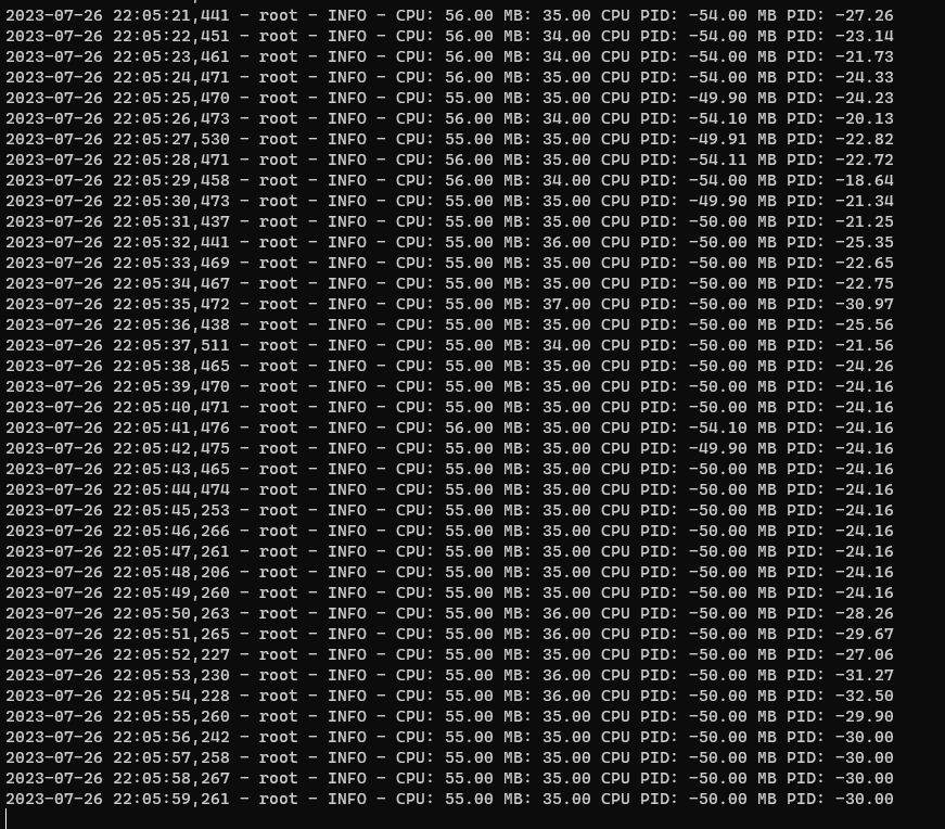
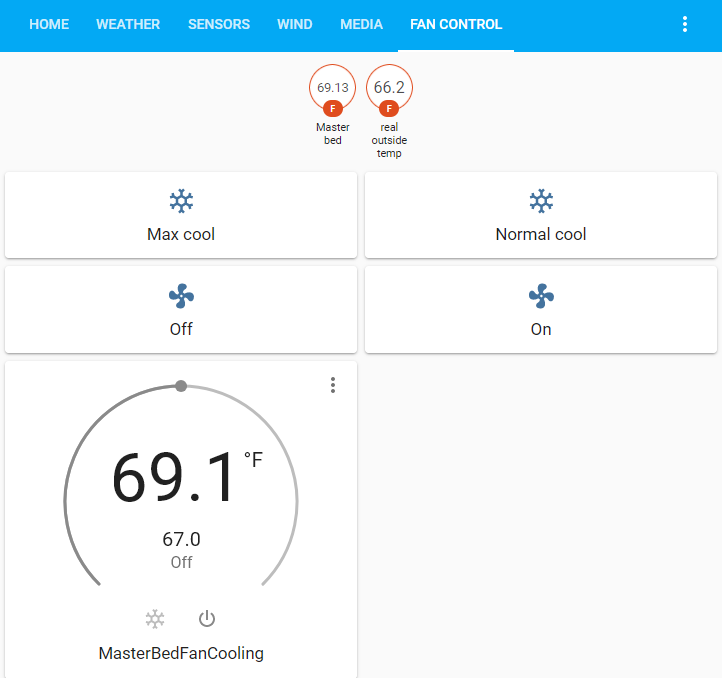
Without further ado: here’s what the super basic dashboard looks like
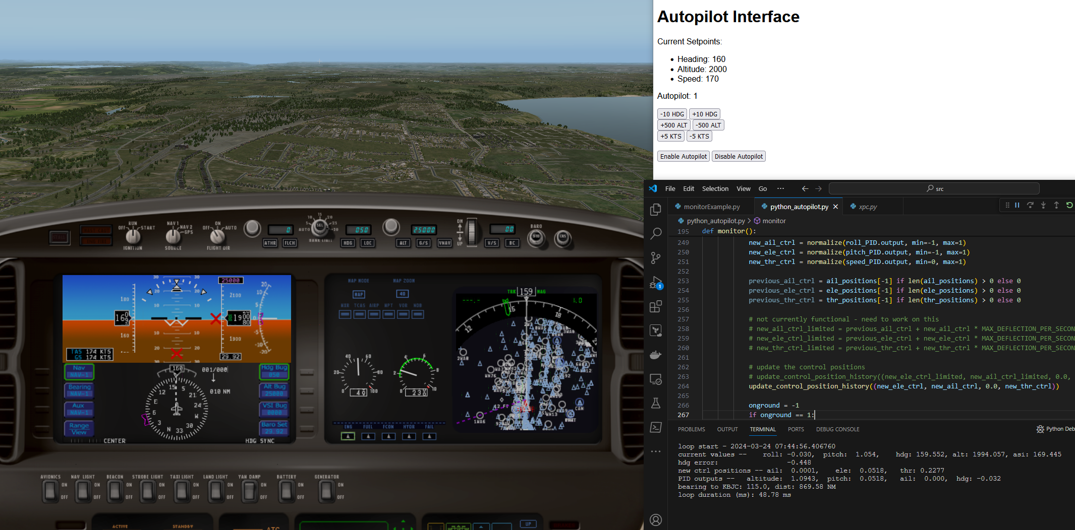
I have it separated into two main running python programs, the file that interacts with X-Plane itself, and the Flask part.
Check here for the updated code / next iteration where I add track following and direct-to functionality – Adding track following (Direct To) with cross track error to the Python X-Plane Autopilot.
Here’s the adjusted autopilot code to check with Redis for the setpoints every loop execution:
# https://onion.io/2bt-pid-control-python/
# https://github.com/ivmech/ivPID

import sys
import os
import xpc
from datetime import datetime, timedelta
import PID
import time
import math, numpy
import redis

r = redis.StrictRedis(host='localhost', port=6379, db=0)

setpoints = {
	"desired_roll": 0,
	"desired_pitch": 2,
	"desired_speed": 160,
	"desired_alt": 8000.0,
	"desired_hdg": 140,
	"autopilot_enabled": 0
}

for key in setpoints:
	# if the key exists in the redis db, use it
	# otherwise, set it
	if r.exists(key):
		setpoints[key] = float(r.get(key))
	else:
		r.set(key, setpoints[key])

update_interval = 0.10 #seconds
update_frequency = 1/update_interval

P = 0.05
I = 0.01
D = 0
MAX_DEFLECTION_PER_SECOND = 2.0

roll_PID = PID.PID(P*2, I*2, D)
roll_PID.SetPoint = setpoints["desired_roll"]

pitch_PID = PID.PID(P, I, D)
pitch_PID.SetPoint = setpoints["desired_pitch"]

altitude_PID = PID.PID(P*2, P/2, D)
altitude_PID.SetPoint = setpoints["desired_alt"]

speed_PID = PID.PID(P, I, D)
speed_PID.SetPoint = setpoints["desired_speed"]

heading_error_PID = PID.PID(1,0.05,0.1)
heading_error_PID.SetPoint = 0 # need heading error to be 0

DREFs = ["sim/cockpit2/gauges/indicators/airspeed_kts_pilot",
		"sim/cockpit2/gauges/indicators/heading_electric_deg_mag_pilot",
		"sim/flightmodel/failures/onground_any",
		"sim/flightmodel/misc/h_ind"]

def normalize(value, min=-1, max=1):
	if (value > max):
		return max
	elif (value < min):
		return min
	else:
		return value

def sleep_until_next_tick(update_frequency):
    # Calculate the update interval from the frequency
    update_interval = 1.0 / update_frequency

    # Get the current time
    current_time = time.time()

    # Calculate the time remaining until the next tick
    sleep_time = update_interval - (current_time % update_interval)

    # Sleep for the remaining time
    time.sleep(sleep_time)

# https://rosettacode.org/wiki/Angle_difference_between_two_bearings#Python
def get_angle_difference(b1, b2):
	r = (b2 - b1) % 360.0
	# Python modulus has same sign as divisor, which is positive here,
	# so no need to consider negative case
	if r >= 180.0:
		r -= 360.0
	return r

# https://gist.github.com/jeromer/2005586
def get_bearing(pointA, pointB):
    """
    Calculates the bearing between two points.
    The formulae used is the following:
        θ = atan2(sin(Δlong).cos(lat2),
                  cos(lat1).sin(lat2) − sin(lat1).cos(lat2).cos(Δlong))
    :Parameters:
      - `pointA: The tuple representing the latitude/longitude for the
        first point. Latitude and longitude must be in decimal degrees
      - `pointB: The tuple representing the latitude/longitude for the
        second point. Latitude and longitude must be in decimal degrees
    :Returns:
      The bearing in degrees
    :Returns Type:
      float
    """
    if (type(pointA) != tuple) or (type(pointB) != tuple):
        raise TypeError("Only tuples are supported as arguments")

    lat1 = math.radians(pointA[0])
    lat2 = math.radians(pointB[0])

    diffLong = math.radians(pointB[1] - pointA[1])

    x = math.sin(diffLong) * math.cos(lat2)
    y = math.cos(lat1) * math.sin(lat2) - (math.sin(lat1)
            * math.cos(lat2) * math.cos(diffLong))

    initial_bearing = math.atan2(x, y)

    # Now we have the initial bearing but math.atan2 return values
    # from -180° to + 180° which is not what we want for a compass bearing
    # The solution is to normalize the initial bearing as shown below
    initial_bearing = math.degrees(initial_bearing)
    compass_bearing = (initial_bearing + 360) % 360

    return compass_bearing

# https://janakiev.com/blog/gps-points-distance-python/
def haversine(coord1, coord2):
    R = 6372800  # Earth radius in meters
    lat1, lon1 = coord1
    lat2, lon2 = coord2

    phi1, phi2 = math.radians(lat1), math.radians(lat2)
    dphi       = math.radians(lat2 - lat1)
    dlambda    = math.radians(lon2 - lon1)

    a = math.sin(dphi/2)**2 + \
        math.cos(phi1)*math.cos(phi2)*math.sin(dlambda/2)**2

    return 2*R*math.atan2(math.sqrt(a), math.sqrt(1 - a))

KBJC_lat = 39.9088056
KBJC_lon = -105.1171944

def write_position_to_redis(position):
	# position is a list of 7 floats
	# position_elements = [lat, lon, alt, pitch, roll, yaw, gear_indicator]
	position_elements = ["lat", "lon", "alt", "pitch", "roll", "yaw", "gear_indicator"]
	position_str = ','.join([str(x) for x in position])
	r.set('position', position_str)
	for i in range(len(position_elements)):
		r.set(f"position/{position_elements[i]}", position[i])

	# position_str = ','.join([str(x) for x in position])
	# r.publish('position_updates', position_str)

def get_setpoints_from_redis():
	setpoints = {
		"desired_roll": 0,
		"desired_pitch": 2,
		"desired_speed": 160,
		"desired_alt": 8000.0,
		"desired_hdg": 140
	}
	for key in setpoints:
		# if the key exists in the redis db, use it
		# otherwise, set it
		if r.exists(key):
			setpoints[key] = float(r.get(key))
		else:
			r.set(key, setpoints[key])
	return setpoints

def get_autopilot_enabled_from_redis():
	if r.exists("autopilot_enabled"):
		return int(r.get("autopilot_enabled").decode('utf-8')) == 1

ele_positions = []
ail_positions = []
thr_positions = []

def update_control_position_history(ctrl):
	ele_positions.append(ctrl[0])
	ail_positions.append(ctrl[1])
	thr_positions.append(ctrl[3])

	# if the list is longer than 20, pop the first element
	if len(ele_positions) > 20:
		ele_positions.pop(0)
		ail_positions.pop(0)
		thr_positions.pop(0)

def monitor():
	with xpc.XPlaneConnect() as client:
		while True:
			loop_start = datetime.now()
			print(f"loop start - {loop_start}")
			posi = client.getPOSI()
			write_position_to_redis(posi)

			ctrl = client.getCTRL()

			bearing_to_kbjc = get_bearing((posi[0], posi[1]), (KBJC_lat, KBJC_lon))
			dist_to_kbjc = haversine((posi[0], posi[1]), (KBJC_lat, KBJC_lon))
			#desired_hdg = 116 #bearing_to_kbjc

			multi_DREFs = client.getDREFs(DREFs) #speed=0, mag hdg=1, onground=2

			current_roll = posi[4]
			current_pitch = posi[3]
			#current_hdg = posi[5] # this is true, need to use DREF to get mag ''
			current_hdg = multi_DREFs[1][0]
			current_altitude = multi_DREFs[3][0]
			current_asi = multi_DREFs[0][0]
			onground = multi_DREFs[2][0]

			# get the setpoints from redis
			setpoints = get_setpoints_from_redis()
			desired_hdg = setpoints["desired_hdg"]
			desired_alt = setpoints["desired_alt"]
			desired_speed = setpoints["desired_speed"]

			# outer loops first
			altitude_PID.SetPoint = desired_alt
			altitude_PID.update(current_altitude)

			heading_error = get_angle_difference(desired_hdg, current_hdg)
			heading_error_PID.update(heading_error)

			speed_PID.SetPoint = desired_speed


			new_pitch_from_altitude = normalize(altitude_PID.output, -10, 10)
			new_roll_from_heading_error = normalize(heading_error_PID.output, -25, 25)
			# if new_pitch_from_altitude > 15:
			# 	new_pitch_from_altitude = 15
			# elif new_pitch_from_altitude < -15:
			# 	new_pitch_from_altitude = -15

			pitch_PID.SetPoint = new_pitch_from_altitude
			roll_PID.SetPoint = new_roll_from_heading_error

			roll_PID.update(current_roll)
			speed_PID.update(current_asi)
			pitch_PID.update(current_pitch)

			new_ail_ctrl = normalize(roll_PID.output, min=-1, max=1)
			new_ele_ctrl = normalize(pitch_PID.output, min=-1, max=1)
			new_thr_ctrl = normalize(speed_PID.output, min=0, max=1)

			previous_ail_ctrl = ail_positions[-1] if len(ail_positions) > 0 else 0
			previous_ele_ctrl = ele_positions[-1] if len(ele_positions) > 0 else 0
			previous_thr_ctrl = thr_positions[-1] if len(thr_positions) > 0 else 0

			# not currently functional - need to work on this
			# new_ail_ctrl_limited = previous_ail_ctrl + new_ail_ctrl * MAX_DEFLECTION_PER_SECOND / update_frequency
			# new_ele_ctrl_limited = previous_ele_ctrl + new_ele_ctrl * MAX_DEFLECTION_PER_SECOND / update_frequency
			# new_thr_ctrl_limited = previous_thr_ctrl + new_thr_ctrl * MAX_DEFLECTION_PER_SECOND / update_frequency

			# update the control positions
			# update_control_position_history((new_ele_ctrl_limited, new_ail_ctrl_limited, 0.0, new_thr_ctrl_limited))
			update_control_position_history((new_ele_ctrl, new_ail_ctrl, 0.0, new_thr_ctrl))

			onground = -1
			if onground == 1:
				print("on ground, not sending controls")
			else:
				if get_autopilot_enabled_from_redis():
					# ctrl = [new_ele_ctrl_limited, new_ail_ctrl_limited, 0.0, new_thr_ctrl_limited]
					ctrl = [new_ele_ctrl, new_ail_ctrl, 0.0, new_thr_ctrl]
					client.sendCTRL(ctrl)

			loop_end = datetime.now()
			loop_duration = loop_end - loop_start

			output = f"current values --    roll: {current_roll: 0.3f},  pitch: {current_pitch: 0.3f},    hdg: {current_hdg:0.3f}, alt: {current_altitude:0.3f}, asi: {current_asi:0.3f}"
			output = output + "\n" + f"hdg error:                 {heading_error: 0.3f}"
			output = output + "\n" + f"new ctrl positions -- ail: {new_ail_ctrl: 0.4f},    ele: {new_ele_ctrl: 0.4f},   thr: {new_thr_ctrl:0.4f}"
			output = output + "\n" + f"PID outputs --   altitude: {altitude_PID.output: 0.4f},  pitch: {pitch_PID.output: 0.4f},   ail: {roll_PID.output: 0.3f},  hdg: {heading_error_PID.output: 0.3f}"
			output = output + "\n" + f"bearing to KBJC: {bearing_to_kbjc:3.1f}, dist: {dist_to_kbjc*0.000539957:0.2f} NM"
			output = output + "\n" + f"loop duration (ms): {loop_duration.total_seconds()*1000:0.2f} ms"
			print(output)
			sleep_until_next_tick(update_frequency)
			os.system('cls' if os.name == 'nt' else 'clear')


if __name__ == "__main__":
	monitor()
And the flask backend/front end. WebSockets are super cool – never used them before this. I was thinking I’d have to make a bunch of endpoints for every type of autopilot change I need. But this handles it far nicer:
from flask import Flask, render_template
from flask_socketio import SocketIO, emit
import redis

app = Flask(__name__)
socketio = SocketIO(app)
r = redis.StrictRedis(host='localhost', port=6379, db=0)

setpoints_of_interest = ['desired_hdg', 'desired_alt', 'desired_speed']
# get initial setpoints from Redis, send to clients

@app.route('/')
def index():
    return render_template('index.html')  # You'll need to create an HTML template

def update_setpoint(label, adjustment):
    # This function can be adapted to update setpoints and then emit updates via WebSocket
    current_value = float(r.get(label)) if r.exists(label) else 0.0

    if label == 'desired_hdg':
        new_value = (current_value + adjustment) % 360
    elif label == 'autopilot_enabled':
        new_value = adjustment
    else:
        new_value = current_value + adjustment

    r.set(label, new_value)
    # socketio.emit('update_setpoint', {label: new_value})  # Emit update to clients
    return new_value

@socketio.on('adjust_setpoint')
def handle_adjust_setpoint(json):
    label = json['label']
    adjustment = json['adjustment']
    # Your logic to adjust the setpoint in Redis and calculate new_value
    new_value = update_setpoint(label, adjustment)

    # Emit updated setpoint to all clients
    emit('update_setpoint', {label: new_value}, broadcast=True)

@socketio.on('connect')
def handle_connect():
    # Fetch initial setpoints from Redis
    initial_setpoints = {label: float(r.get(label)) if r.exists(label) else 0.0 for label in setpoints_of_interest}

    # Emit the initial setpoints to the connected client
    emit('update_setpoints', initial_setpoints)

if __name__ == '__main__':
    socketio.run(app)
And the http template:
<!DOCTYPE html>
<html>
<head>
    <title>Autopilot Interface</title>
    <script src="https://cdnjs.cloudflare.com/ajax/libs/socket.io/4.0.1/socket.io.js"></script>
<script type="text/javascript" charset="utf-8">
    var socket;  // Declare socket globally

    // Define adjustSetpoint globally
    function adjustSetpoint(label, adjustment) {
        socket.emit('adjust_setpoint', {label: label, adjustment: adjustment});
    }

    document.addEventListener('DOMContentLoaded', () => {
        socket = io.connect(location.protocol + '//' + document.domain + ':' + location.port);

        socket.on('connect', () => {
            console.log("Connected to WebSocket server.");
        });

        // Listen for update_setpoints event to initialize the UI with Redis values
        socket.on('update_setpoints', function(setpoints) {
          for (const [label, value] of Object.entries(setpoints)) {
              const element = document.getElementById(label);
              if (element) {
                  element.innerHTML = value;
              }
          }
      });

        // Listen for update_setpoint events from the server
        socket.on('update_setpoint', data => {
            // Assuming 'data' is an object like {label: new_value}
            for (const [label, value] of Object.entries(data)) {
                // Update the displayed value on the webpage
                const element = document.getElementById(label);
                if (element) {
                    element.innerHTML = value;
                }
            }
        });
    });
</script>

</head>
<body>
    <h1>Autopilot Interface</h1>
    <p>Current Setpoints:</p>
    <ul>
        <li>Heading: <span id="desired_hdg">0</span></li>
        <li>Altitude: <span id="desired_alt">0</span></li>
        <li>Speed: <span id="desired_speed">0</span></li>
    </ul>
    <p>Autopilot: <span id="autopilot_enabled">0</span></p>

    <!-- Example buttons for adjusting setpoints -->
    <button onclick="adjustSetpoint('desired_hdg', -10)">-10 HDG</button>
    <button onclick="adjustSetpoint('desired_hdg', 10)">+10 HDG</button>
    <br>
    <button onclick="adjustSetpoint('desired_alt', 500)">+500 ALT</button>
    <button onclick="adjustSetpoint('desired_alt', -500)">-500 ALT</button>
    <br>
    <button onclick="adjustSetpoint('desired_speed', 5)">+5 KTS</button>
    <button onclick="adjustSetpoint('desired_speed', -5)">-5 KTS</button>
    <br>
    <br>
    <button onclick="adjustSetpoint('autopilot_enabled', 1)">Enable Autopilot</button>
    <button onclick="adjustSetpoint('autopilot_enabled', 0)">Disable Autopilot</button>

</body>
</html>
This should be enough to get you going. I’ll come back and clean it up later (both my kids just woke up – 1.5 and 3.5 years!)