Introduction
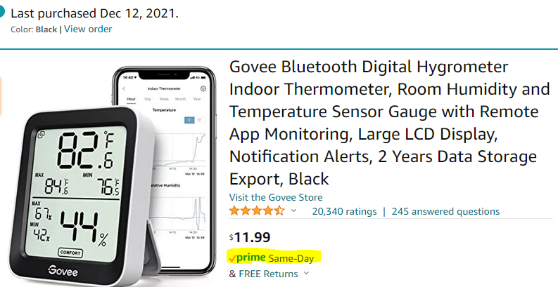
Like many other Home Automation enthusiasts, I have been on the lookout for a cheap thermometer/hygrometer that has either WiFi or Bluetooth connectivity. I think I found the answer in the $12 USD Govee Bluetooth Digital Thermometer and Hygrometer. The fact that the device broadcasts the current temperature and humidity every 2 seconds via low energy Bluetooth (BLE) is the metaphorical icing on the cake. Here is a pic of the unit in our garage:

Specifications
This is a pretty basic device. It has a screen that shows the current temperature, humidity, and min/max values. It sends the current readings (along with battery health) every 2 seconds via low-energy bluetooth (BLE). The description on Amazon says it has a “Swiss-made smart hygrometer sensor”. Dunno if I believe that but for $12 it is good enough. The temperature is accurate to +/- 0.54F and humidity is +/- 3% RH. If you use the app, it is apparently possible to read the last 20 days or 2 years of data from the device (I haven’t used the app at all).
Enough with the boring stuff. Let’s get it connected to Home Assistant.
Reading the Govee bluetooth advertisements with Python
I found some sample code on tchen’s GitHub page (link) to help get me going in the right direction.
Without further ado, here is the code I’m using to read the data and publish via MQTT:
observe.py (updated 2022-01-04 with some logging improvements. default logging level is now WARNING, which disables printing every advertisement)
# basic govee bluetooth data reading code for model https://amzn.to/3z14BIi
# written/modified by Austin of austinsnerdythings.com 2021-12-27
# original source: https://gist.github.com/tchen/65d6b29a20dd1ef01b210538143c0bf4
import logging
import json
from time import sleep
from basic_mqtt import basic_mqtt
from bleson import get_provider, Observer

logging.basicConfig(
	format='%(asctime)s.%(msecs)03d - %(name)s - %(levelname)s - %(message)s',
	datefmt='%Y-%m-%d %H:%M:%S',
	level=logging.WARNING)

# I did write all the mqtt stuff. I kept it in a separate class
mqtt = basic_mqtt()
mqtt.connect()

# writing code on my windows computer, committing, pushing, and then
# pulling the new code on the Raspberry Pi is a tedious "debug" process.
# there are quite a few errors that spit out from bleson, which as far
# as I can tell, isn't super polished. if we set the debug level to
# critical, most of those disappear.
logging.getLogger("bleson").setLevel(logging.CRITICAL)

# basic celsius to fahrenheit function
def c2f(val):
    return round(32 + 9*val/5, 2)

last = {}

# I didn't write this, but it takes the raw BT data and spits out the data of interest
def temp_hum(values, battery, address):
    global last
    #########################
    #
    # there is a fix for temperatures below freezing here -
    # https://github.com/joshgordon/govee_ble_to_mqtt/blob/master/observe.py
    # I will adjust post code afternoon of 2022-11-28
    #
    #########################
    values = int.from_bytes(values, 'big')
    if address not in last or last[address] != values:
        last[address] = values
        temp = float(values / 10000)
        hum = float((values % 1000) / 10)
        # this print looks like this:
        # 2021-12-27T11:22:17.040469 BDAddress('A4:C1:38:9F:1B:A9') Temp: 45.91 F  Humidity: 25.8 %  Battery: 100 %
        logging.info(f"decoded values: {address} Temp: {c2f(temp)} F  Humidity: {hum} %  Battery: {battery}")
        # this code originally just printed the data, but we need it to publish to mqtt.
        # added the return values to be used elsewhere
        return c2f(temp), hum, battery

def on_advertisement(advertisement):
    #print(advertisement)
    mfg_data = advertisement.mfg_data

    # there are lots of BLE advertisements flying around. only look at ones that have mfg_data
    if mfg_data is not None:
        #print(advertisement)
        # there are a few Govee models and the data is in different positions depending on which
        # the unit of interest isn't either of these hardcoded values, so they are skipped
        if advertisement.name == 'GVH5177_9835':
            address = advertisement.address
            temp_hum(mfg_data[4:7], mfg_data[7], address)
        elif advertisement.name == 'GVH5075_391D':
            address = advertisement.address
            temp_hum(mfg_data[3:6], mfg_data[6], address)
        elif advertisement.name != None:
            # this is where all of the advertisements for our unit of interest will be processed
            address = advertisement.address
            if 'GVH' in advertisement.name:
                #print(advertisement)
                temp_f, hum, battery = temp_hum(mfg_data[3:6], mfg_data[6], address)

                if temp_f > 180.0 or temp_f < -30.0:
                    return
                # as far as I can tell bleson doesn't have a string representation of the MAC address
                # address is of type BDAddress(). str(address) is BDAddress('A4:C1:38:9F:1B:A9')
                # substring 11:-2 is just the MAC address
                mac_addr = str(address)[11:-2]

                # construct dict with relevant info
                msg = {'temp_f':temp_f,
                        'hum':hum,
                        'batt':battery}

                # looks like this:
                # msg data: {'temp_f': 45.73, 'hum': 25.5, 'batt': 100}
                logging.info(f"MQTT msg data: {msg}")

                # turn into JSON for publishing
                json_string = json.dumps(msg, indent=4)

                # publish to topic separated by MAC address
                mqtt.publish(f"govee/{mac_addr}", json_string)

# base stuff from the original gist
logging.warning(f"initializing bluetooth")
adapter = get_provider().get_adapter()
observer = Observer(adapter)
observer.on_advertising_data = on_advertisement

logging.warning(f"starting observer")
observer.start()
logging.warning(f"listening for events and publishing to MQTT")
while True:
    # unsure about this loop and how much of a delay works
    sleep(1)
observer.stop()
And for the MQTT helper class (mqtt_helper.py):
# basic MQTT helper class. really needed to write one of these to simplify basic MQTT operations
# written/modified by Austin of austinsnerdythings.com 2021-12-27
# original source: https://gist.github.com/fisherds/f302b253cf7a11c2a0d814acd424b9bb
# filename is basic_mqtt.py
from paho.mqtt import client as mqtt_client
import logging
import datetime
logging.basicConfig(
	format='%(asctime)s.%(msecs)03d - %(name)s - %(levelname)s - %(message)s',
	datefmt='%Y-%m-%d %H:%M:%S',
	level=logging.INFO)


mqtt_host = "mqtt.home.fluffnet.net"
test_topic = "mqtt_test_topic"

# this is really not polished. it was a stream of consciousness project to pound
# something out to do basic MQTT publish stuff in a reusable fashion.
class basic_mqtt:
	def __init__(self):
		self.client = mqtt_client.Client()
		self.subscription_topic_name = None
		self.publish_topic_name = None
		self.callback = None
		self.host = mqtt_host

	def connect(self):
		self.client.on_connect = self.on_connect
		self.client.on_subscribe = self.on_subscribe
		self.client.on_message = self.on_message
		logging.info(f"connecting to MQTT broker at {mqtt_host}")
		self.client.connect(host=mqtt_host,keepalive=30)
		self.client.loop_start()

	def on_connect(self, client, userdata, flags, rc):
		print("Connected with result code "+str(rc))

		# Subscribing in on_connect() means that if we lose the connection and
		# reconnect then subscriptions will be renewed.
		#self.client.subscribe("$SYS/#")

	def on_message(self, client, userdata, msg):
		print(f"got message of topic {msg.topic} with payload {msg.payload}")

	def on_subscribe(self, client, userdata, mid, granted_qos):
		print("Subscribed: " + str(mid) + " " + str(granted_qos))

	def publish(self, topic, msg):
		self.client.publish(topic=topic, payload=msg)

	def subscribe_to_test_topic(self, topic=test_topic):
		self.client.subscribe(topic)

	def send_test_message(self, topic=test_topic):

		self.publish(topic=topic, msg=f"test message from python script at {datetime.datetime.now()}")

	def disconnect(self):
		self.client.disconnect()

	def loop(self):
		self.client.loop_forever()

if __name__ == "__main__":
	logging.info("running MQTT test")
	mqtt_helper = basic_mqtt()
	mqtt_helper.connect()
	mqtt_helper.subscribe_to_test_topic()
	mqtt_helper.send_test_message()
	mqtt_helper.disconnect()
Results
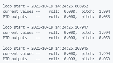
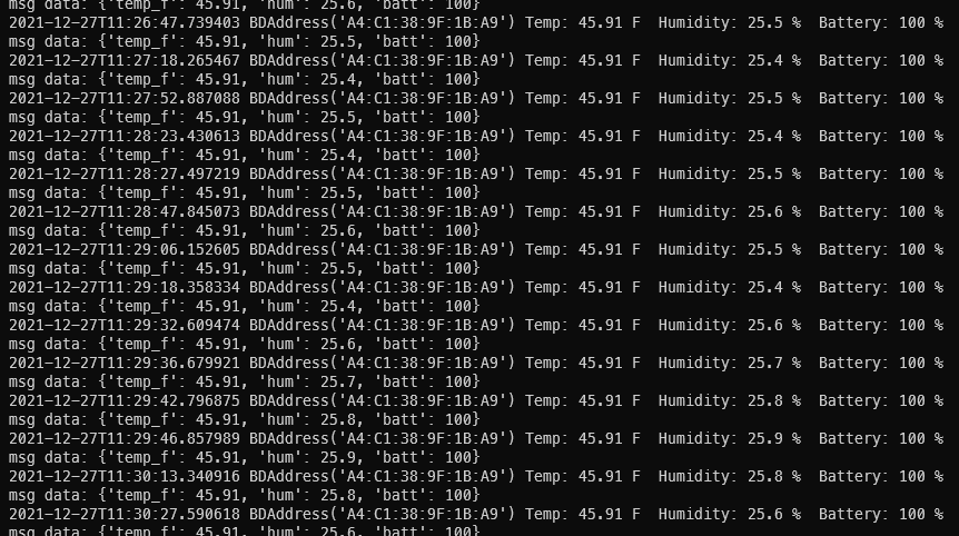
Running this script on a Raspberry Pi 3 shows the advertisements coming in as expected. The updates are very quick compared to the usual 16 second update interval for my Acurite stuff.
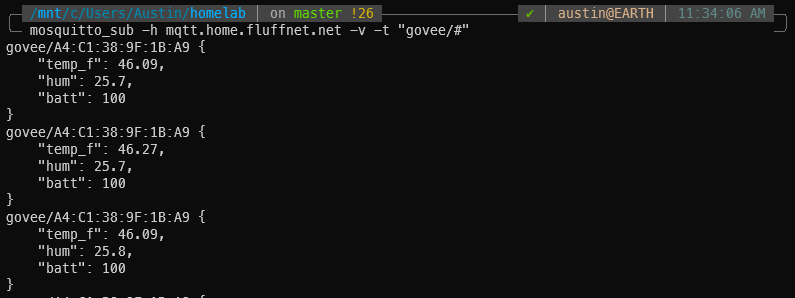
And running mosquitto_sub with the right arguments (mosquitto_sub -h mqtt -v -t “govee/#”) shows the MQTT messages are being published as expected:
Getting Govee MQTT data into Home Assistant
Lastly, we need to add a MQTT sensor to get the data importing into Home Assistant:
- platform: mqtt
  state_topic: "govee/A4:C1:38:9F:1B:A9"
  value_template: "{{ value_json.temp_f }}"
  name: "garage temp"
  unit_of_measurement: "F"
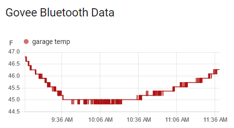
And from there you can do whatever you want with the collected data!
Conclusion
This was a relatively quick post and code development. I really hate the cycle of developing on my Bluetooth-less Windows computer, committing the code, pushing to Git, pulling on the Pi, and running to “debug”. Thus, the code isn’t as good as it can be. I probably did 20-25 iterations before calling it good enough.
Regardless, I think this $12 Govee Bluetooth Thermometer and Hygrometer is a great little tool for collecting data around the house. You don’t need an SDR to get Acurite beacons, and you don’t need to spend a lot either. You just need a way to receive BLE advertisements (basically any Bluetooth-capable device can do this). There is even a 2 pack of just the sensors that I just discovered on Amazon for $24 – 2 pack of Govee bluetooth thermometer and hygrometer. I know there are other Bluetooth devices but they’re quite a bit more expensive.
Disclosure: Some of the links on this post are Amazon affiliate links. This means that, at zero cost to you, I will earn an affiliate commission if you click through the link and finalize a purchase.
Also, at least for me, these are available with same day shipping on Amazon. Scratch that instant gratification itch.